Multiclass predictive modeling for #TidyTuesday NBER papers

This is the latest in my series of screencasts demonstrating how to use the tidymodels packages, from just getting started to tuning more complex models. Today’s screencast walks through how to build, tune, and evaluate a multiclass predictive model with text features and lasso regularization, with this week’s #TidyTuesday dataset on NBER working papers. 📑

Here is the code I used in the video, for those who prefer reading instead of or in addition to video.

Explore data

Our modeling goal is to predict the category of National Bureau of Economic Research working papers from the titles and years of the papers.

library(tidyverse)

papers <- readr::read_csv("https://raw.githubusercontent.com/rfordatascience/tidytuesday/master/data/2021/2021-09-28/papers.csv")
programs <- readr::read_csv("https://raw.githubusercontent.com/rfordatascience/tidytuesday/master/data/2021/2021-09-28/programs.csv")
paper_authors <- readr::read_csv("https://raw.githubusercontent.com/rfordatascience/tidytuesday/master/data/2021/2021-09-28/paper_authors.csv")
paper_programs <- readr::read_csv("https://raw.githubusercontent.com/rfordatascience/tidytuesday/master/data/2021/2021-09-28/paper_programs.csv")

Let’s start by joining up these datasets to find the info we need.

papers_joined <-
  paper_programs %>%
  left_join(programs) %>%
  left_join(papers) %>%
  filter(!is.na(program_category)) %>%
  distinct(paper, program_category, year, title)

papers_joined %>%
  count(program_category)

## # A tibble: 3 × 2
##   program_category        n
##   <chr>               <int>
## 1 Finance              4336
## 2 Macro/International 12012
## 3 Micro               18527

The papers are in three categories (finance, microeconomics, and macroeconomics) so we’ll be training a multiclass predictive model, not a binary classification model as we often see or use.

Let’s create one exploratory plot before we move on to modeling.

library(tidytext)
library(tidylo)

title_log_odds <-
  papers_joined %>%
  unnest_tokens(word, title) %>%
  filter(!is.na(program_category)) %>%
  count(program_category, word, sort = TRUE) %>%
  bind_log_odds(program_category, word, n)


title_log_odds %>%
  group_by(program_category) %>%
  slice_max(log_odds_weighted, n = 10) %>%
  ungroup() %>%
  ggplot(aes(log_odds_weighted,
    fct_reorder(word, log_odds_weighted),
    fill = program_category
  )) +
  geom_col(show.legend = FALSE) +
  facet_wrap(vars(program_category), scales = "free_y") +
  labs(x = "Log odds (weighted)", y = NULL)

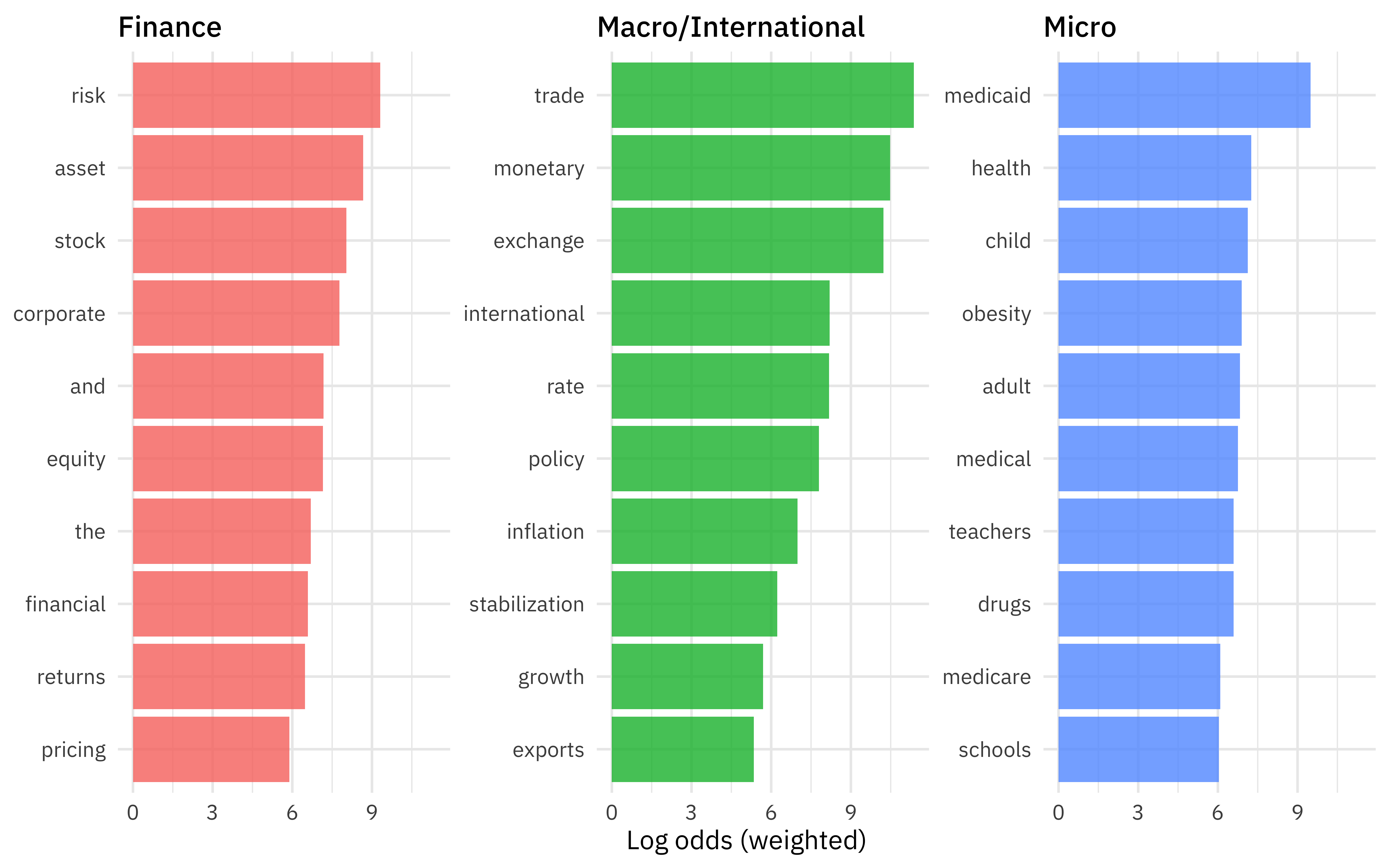
These type of relationships between category and title words are what we want to use in our predictive model.

Build and tune a model

Let’s start our modeling by setting up our “data budget.” We’ll stratify by our outcome program_category.

library(tidymodels)

set.seed(123)
nber_split <- initial_split(papers_joined, strata = program_category)
nber_train <- training(nber_split)
nber_test <- testing(nber_split)

set.seed(234)
nber_folds <- vfold_cv(nber_train, strata = program_category)
nber_folds

## #  10-fold cross-validation using stratification 
## # A tibble: 10 × 2
##    splits               id    
##    <list>               <chr> 
##  1 <split [23539/2617]> Fold01
##  2 <split [23539/2617]> Fold02
##  3 <split [23540/2616]> Fold03
##  4 <split [23540/2616]> Fold04
##  5 <split [23540/2616]> Fold05
##  6 <split [23541/2615]> Fold06
##  7 <split [23541/2615]> Fold07
##  8 <split [23541/2615]> Fold08
##  9 <split [23541/2615]> Fold09
## 10 <split [23542/2614]> Fold10

Next, let’s set up our feature engineering. We will need to transform our text data into features useful for our model by tokenizing and computing (in this case) tf-idf. Let’s also downsample since our dataset is imbalanced, with many more of some of the categories than others.

library(themis)
library(textrecipes)

nber_rec <-
  recipe(program_category ~ year + title, data = nber_train) %>%
  step_tokenize(title) %>%
  step_tokenfilter(title, max_tokens = 200) %>%
  step_tfidf(title) %>%
  step_downsample(program_category)

nber_rec

## Recipe
## 
## Inputs:
## 
##       role #variables
##    outcome          1
##  predictor          2
## 
## Operations:
## 
## Tokenization for title
## Text filtering for title
## Term frequency-inverse document frequency with title
## Down-sampling based on program_category

Then, let’s create our model specification for a lasso model. We need to use a model specification that can handle multiclass data, in this case multinom_reg().

multi_spec <-
  multinom_reg(penalty = tune(), mixture = 1) %>%
  set_mode("classification") %>%
  set_engine("glmnet")

multi_spec

## Multinomial Regression Model Specification (classification)
## 
## Main Arguments:
##   penalty = tune()
##   mixture = 1
## 
## Computational engine: glmnet

Now it’s time to put the preprocessing and model together in a workflow().

nber_wf <- workflow(nber_rec, multi_spec)
nber_wf

## ══ Workflow ════════════════════════════════════════════════════════════════════
## Preprocessor: Recipe
## Model: multinom_reg()
## 
## ── Preprocessor ────────────────────────────────────────────────────────────────
## 4 Recipe Steps
## 
## • step_tokenize()
## • step_tokenfilter()
## • step_tfidf()
## • step_downsample()
## 
## ── Model ───────────────────────────────────────────────────────────────────────
## Multinomial Regression Model Specification (classification)
## 
## Main Arguments:
##   penalty = tune()
##   mixture = 1
## 
## Computational engine: glmnet

Since the lasso regularization penalty is a hyperparameter of the model (we can’t find the best value from fitting the model a single time), let’s tune over a grid of possible penalty parameters.

nber_grid <- grid_regular(penalty(range = c(-5, 0)), levels = 20)

doParallel::registerDoParallel()
set.seed(2021)
nber_rs <-
  tune_grid(
    nber_wf,
    nber_folds,
    grid = nber_grid
  )

nber_rs

## # Tuning results
## # 10-fold cross-validation using stratification 
## # A tibble: 10 × 4
##    splits               id     .metrics          .notes          
##    <list>               <chr>  <list>            <list>          
##  1 <split [23539/2617]> Fold01 <tibble [40 × 5]> <tibble [0 × 1]>
##  2 <split [23539/2617]> Fold02 <tibble [40 × 5]> <tibble [0 × 1]>
##  3 <split [23540/2616]> Fold03 <tibble [40 × 5]> <tibble [0 × 1]>
##  4 <split [23540/2616]> Fold04 <tibble [40 × 5]> <tibble [0 × 1]>
##  5 <split [23540/2616]> Fold05 <tibble [40 × 5]> <tibble [0 × 1]>
##  6 <split [23541/2615]> Fold06 <tibble [40 × 5]> <tibble [0 × 1]>
##  7 <split [23541/2615]> Fold07 <tibble [40 × 5]> <tibble [0 × 1]>
##  8 <split [23541/2615]> Fold08 <tibble [40 × 5]> <tibble [0 × 1]>
##  9 <split [23541/2615]> Fold09 <tibble [40 × 5]> <tibble [0 × 1]>
## 10 <split [23542/2614]> Fold10 <tibble [40 × 5]> <tibble [0 × 1]>

This is a pretty fast model to fit, since it is linear. How did it turn out?

autoplot(nber_rs)

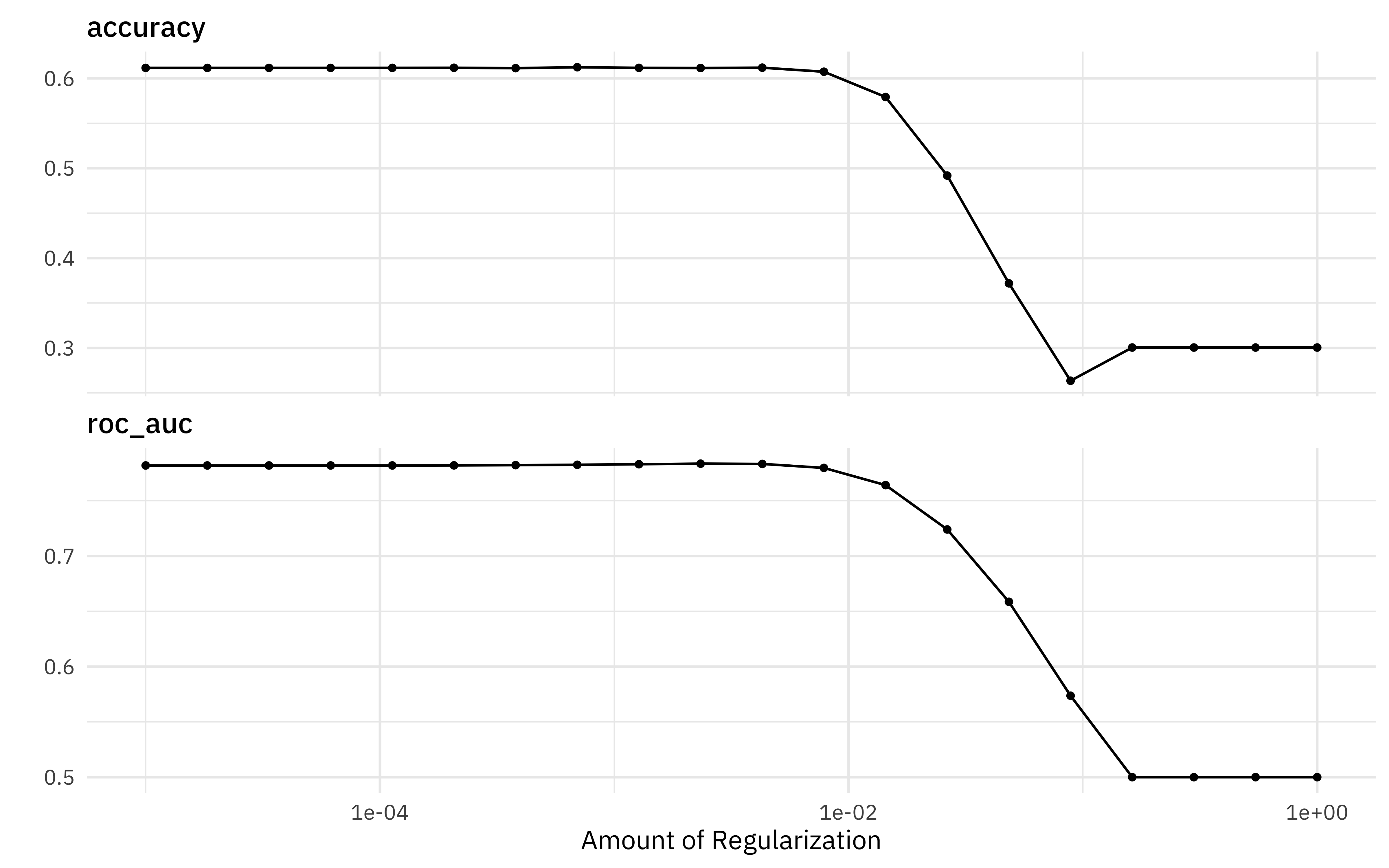
show_best(nber_rs)

## # A tibble: 5 × 7
##    penalty .metric .estimator  mean     n std_err .config              
##      <dbl> <chr>   <chr>      <dbl> <int>   <dbl> <chr>                
## 1 0.00234  roc_auc hand_till  0.784    10 0.00249 Preprocessor1_Model10
## 2 0.00428  roc_auc hand_till  0.783    10 0.00244 Preprocessor1_Model11
## 3 0.00127  roc_auc hand_till  0.783    10 0.00251 Preprocessor1_Model09
## 4 0.000695 roc_auc hand_till  0.782    10 0.00253 Preprocessor1_Model08
## 5 0.000379 roc_auc hand_till  0.782    10 0.00254 Preprocessor1_Model07

Choose and evaluate a final model

We could use the numerically best model with select_best() by often with regularized models we would rather choose a simpler model within some limits of performance. We can choose using the “one-standard error rule” with select_by_one_std_err() and then use last_fit() to fit one time to the training data and evaluate one time to the testing data.

final_penalty <-
  nber_rs %>%
  select_by_one_std_err(metric = "roc_auc", desc(penalty))

final_penalty

## # A tibble: 1 × 9
##   penalty .metric .estimator  mean     n std_err .config            .best .bound
##     <dbl> <chr>   <chr>      <dbl> <int>   <dbl> <chr>              <dbl>  <dbl>
## 1 0.00428 roc_auc hand_till  0.783    10 0.00244 Preprocessor1_Mod… 0.784  0.781

final_rs <-
  nber_wf %>%
  finalize_workflow(final_penalty) %>%
  last_fit(nber_split)

final_rs

## # Resampling results
## # Manual resampling 
## # A tibble: 1 × 6
##   splits               id               .metrics  .notes  .predictions .workflow
##   <list>               <chr>            <list>    <list>  <list>       <list>   
## 1 <split [26156/8719]> train/test split <tibble … <tibbl… <tibble [8,… <workflo…

How did our final model perform on the training data?

collect_metrics(final_rs)

## # A tibble: 2 × 4
##   .metric  .estimator .estimate .config             
##   <chr>    <chr>          <dbl> <chr>               
## 1 accuracy multiclass     0.609 Preprocessor1_Model1
## 2 roc_auc  hand_till      0.779 Preprocessor1_Model1

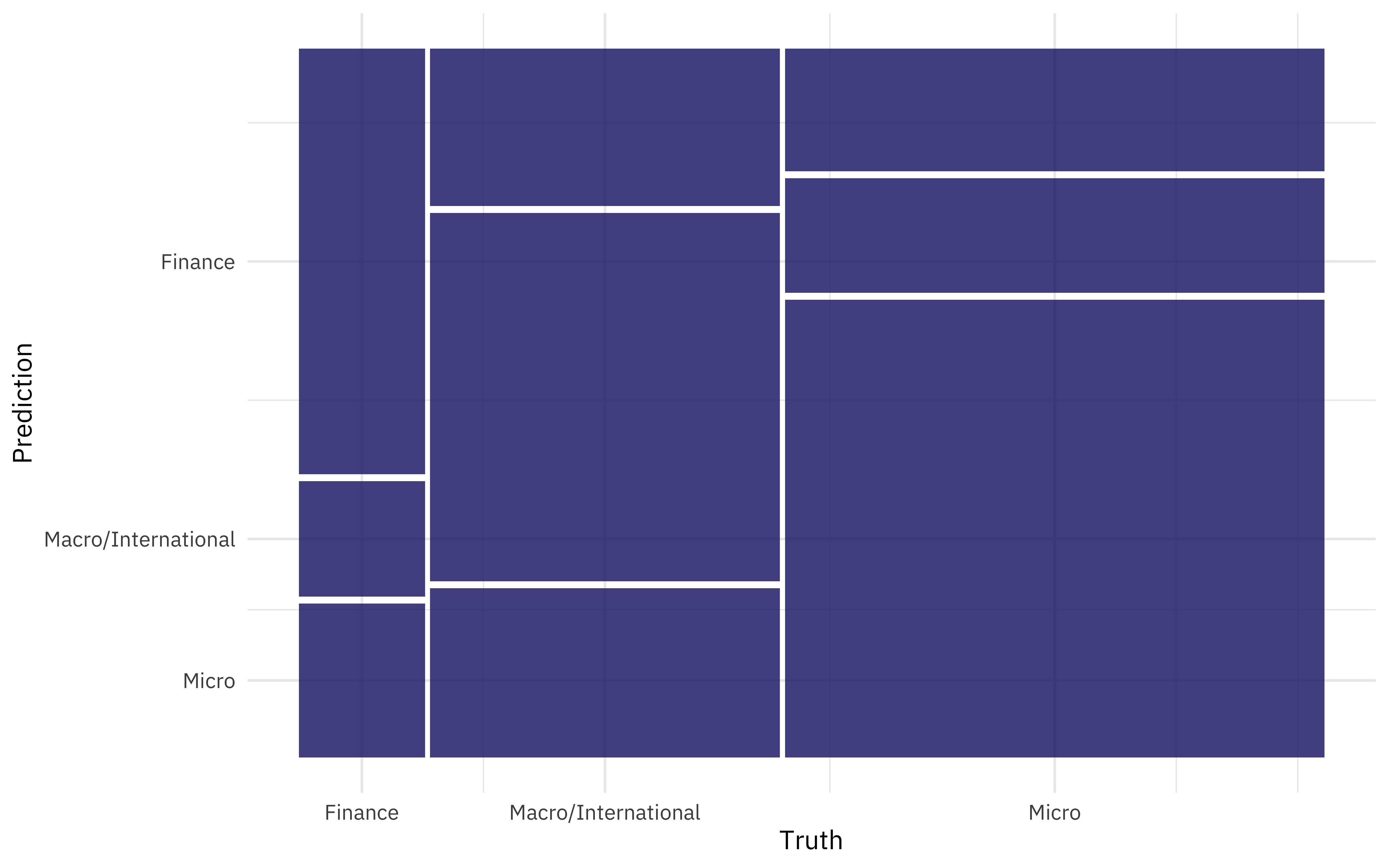
We can visualize the difference in performance across classes with a confusion matrix.

collect_predictions(final_rs) %>%
  conf_mat(program_category, .pred_class) %>%
  autoplot()

We can also visualize the ROC curves for each class.

collect_predictions(final_rs) %>%
  roc_curve(truth = program_category, .pred_Finance:.pred_Micro) %>%
  ggplot(aes(1 - specificity, sensitivity, color = .level)) +
  geom_abline(slope = 1, color = "gray50", lty = 2, alpha = 0.8) +
  geom_path(size = 1.5, alpha = 0.7) +
  labs(color = NULL) +
  coord_fixed()

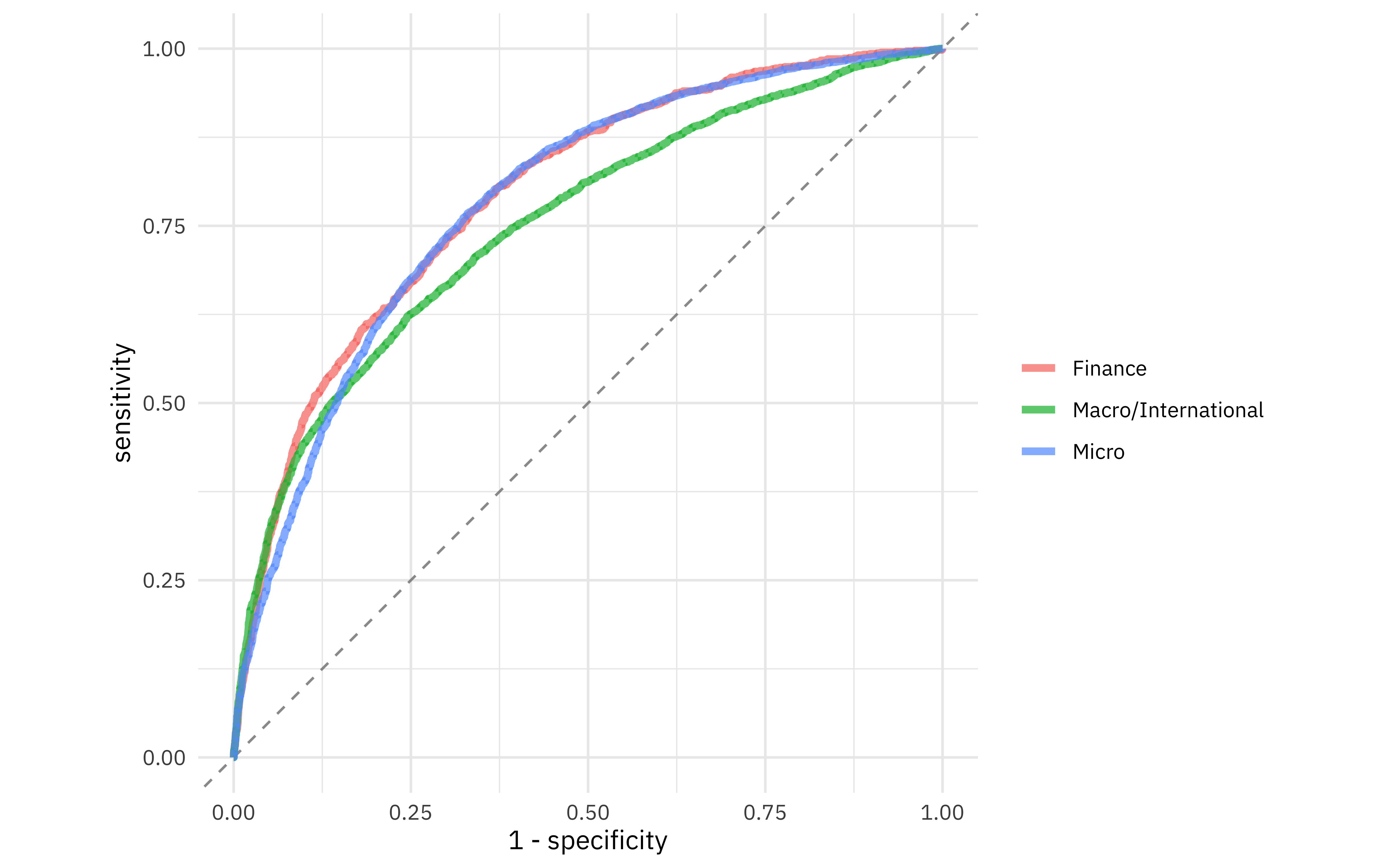
It looks like the finance and microeconomics papers were easier to identify than the macroeconomics papers.

Finally, we can extract (and save, if we like) the fitted workflow from our results to use for predicting on new data.

final_fitted <- extract_workflow(final_rs)
## can save this for prediction later with readr::write_rds()

predict(final_fitted, nber_test[111, ], type = "prob")

## # A tibble: 1 × 3
##   .pred_Finance `.pred_Macro/International` .pred_Micro
##           <dbl>                       <dbl>       <dbl>
## 1         0.104                       0.531       0.365

We can even make up new paper titles and see how our model classifies them.

predict(final_fitted, tibble(year = 2021, title = "Pricing Models for Corporate Responsibility"), type = "prob")

## # A tibble: 1 × 3
##   .pred_Finance `.pred_Macro/International` .pred_Micro
##           <dbl>                       <dbl>       <dbl>
## 1         0.598                       0.158       0.244

predict(final_fitted, tibble(year = 2021, title = "Teacher Health and Medicaid Expansion"), type = "prob")

## # A tibble: 1 × 3
##   .pred_Finance `.pred_Macro/International` .pred_Micro
##           <dbl>                       <dbl>       <dbl>
## 1         0.288                       0.141       0.571