Predicting viewership for #TidyTuesday Doctor Who episodes
By Julia Silge in rstats tidymodels
November 27, 2021
This is the latest in my series of
screencasts demonstrating how to use the
tidymodels packages, from just getting started to tuning more complex models. Today’s screencast walks through how to handle workflow objects, with this week’s
#TidyTuesday dataset on Doctor Who episodes. 💙
Here is the code I used in the video, for those who prefer reading instead of or in addition to video.
Explore data
Our modeling goal is to predict the UK viewership of Doctor Who episodes (since the 2005 revival) from the episodes’ air date. How has the viewership of these episodes changed over time?
episodes <- readr::read_csv("https://raw.githubusercontent.com/rfordatascience/tidytuesday/master/data/2021/2021-11-23/episodes.csv") %>%
  filter(!is.na(uk_viewers))

episodes %>%
  ggplot(aes(first_aired, uk_viewers)) +
  geom_line(alpha = 0.8, size = 1.2, color = "midnightblue") +
  labs(x = NULL)
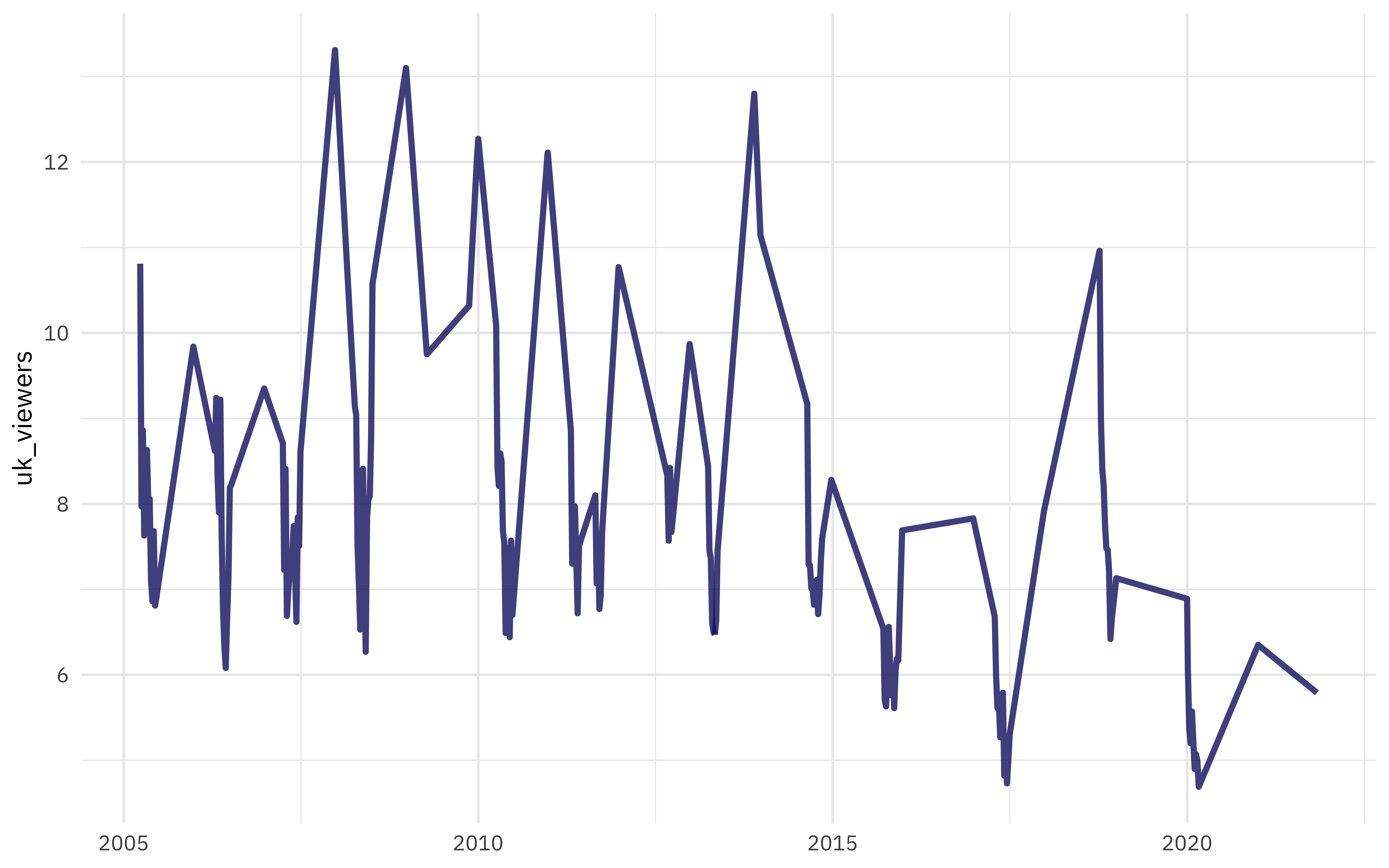
These are quite spiky, with much higher viewer numbers for special episodes like season finales or Christmas episodes.
I have only ever watched episodes of Doctor Who after they arrive on US streaming platforms, but I will say that I haven’t caught up on some of the latest seasons, much like many viewers in the UK.
Create a workflow
In tidymodels, we typically recommend using a workflow in your modeling analyses, to make it easier to carry around preprocessing and modeling components in your code and to protect against errors. Let’s create some bootstrap resampling folds for these episodes, and then a workflow to predict viewership (in millions) from the air date.
library(tidymodels)

set.seed(123)
folds <- bootstraps(episodes, times = 100, strata = uk_viewers)
folds
## # Bootstrap sampling using stratification
## # A tibble: 100 × 2
##    splits           id
##    <list>           <chr>
##  1 <split [167/61]> Bootstrap001
##  2 <split [167/55]> Bootstrap002
##  3 <split [167/64]> Bootstrap003
##  4 <split [167/56]> Bootstrap004
##  5 <split [167/69]> Bootstrap005
##  6 <split [167/63]> Bootstrap006
##  7 <split [167/68]> Bootstrap007
##  8 <split [167/55]> Bootstrap008
##  9 <split [167/60]> Bootstrap009
## 10 <split [167/60]> Bootstrap010
## # … with 90 more rows
We want to use first_aired as our predictor, but let’s do some feature engineering here. Let’s create a date feature (just year here; if we had more data, maybe we could try week of the year or month), and also create a feature for a few holidays that are celebrated in the UK and have special Doctor Who episodes.
who_rec <-
  recipe(uk_viewers ~ first_aired, data = episodes) %>%
  step_date(first_aired, features = "year") %>%
  step_holiday(first_aired,
    holidays = c("NewYearsDay", "ChristmasDay"),
    keep_original_cols = FALSE
  )

## not needed for modeling, but just to check how things are going:
prep(who_rec) %>% bake(new_data = NULL)
## # A tibble: 167 × 4
##    uk_viewers first_aired_year first_aired_NewYearsDay first_aired_ChristmasDay
##         <dbl>            <dbl>                   <dbl>                    <dbl>
##  1      10.8              2005                       0                        0
##  2       7.97             2005                       0                        0
##  3       8.86             2005                       0                        0
##  4       7.63             2005                       0                        0
##  5       7.98             2005                       0                        0
##  6       8.63             2005                       0                        0
##  7       8.01             2005                       0                        0
##  8       8.06             2005                       0                        0
##  9       7.11             2005                       0                        0
## 10       6.86             2005                       0                        0
## # … with 157 more rows
Now let’s combine this feature engineering recipe together with a model. We don’t have much data here, so let’s stick with a straightforward OLS linear model.
who_wf <- workflow(who_rec, linear_reg())
who_wf
## ══ Workflow ════════════════════════════════════════════════════════════════════
## Preprocessor: Recipe
## Model: linear_reg()
##
## ── Preprocessor ────────────────────────────────────────────────────────────────
## 2 Recipe Steps
##
## • step_date()
## • step_holiday()
##
## ── Model ───────────────────────────────────────────────────────────────────────
## Linear Regression Model Specification (regression)
##
## Computational engine: lm
Extract custom quantities from resampled workflows
If you look at many of my tutorials or the documentation for tidymodels, you’ll see that we can fit our workflow to our resamples with code like fit_resamples(who_wf, folds). This can give us some useful results, but sometimes we want more. The functions like fit_resamples() and tune_grid() and friends don’t keep the fitted models they train, because they are all trained for the purpose of evaluation or tuning or similar; we usually throw those models away. Sometimes we want to record something about those models beyond their performance; we can do that using a special control_*() function.
ctrl_extract <- control_resamples(extract = extract_fit_engine)
To create ctrl_extract, I used the
extract_fit_engine() function, but you have total flexibility here and can supply your own function. Check out
this tutorial for another way to supply a custom function here.
With our ctrl_extract ready to go, we can now fit to our resamples and keep the linear models for each resample.
doParallel::registerDoParallel()
set.seed(234)
who_rs <- fit_resamples(who_wf, folds, control = ctrl_extract)
who_rs
## # Resampling results
## # Bootstrap sampling using stratification
## # A tibble: 100 × 5
##    splits           id           .metrics         .notes           .extracts
##    <list>           <chr>        <list>           <list>           <list>
##  1 <split [167/61]> Bootstrap001 <tibble [2 × 4]> <tibble [0 × 1]> <tibble [1 ×…
##  2 <split [167/55]> Bootstrap002 <tibble [2 × 4]> <tibble [0 × 1]> <tibble [1 ×…
##  3 <split [167/64]> Bootstrap003 <tibble [2 × 4]> <tibble [0 × 1]> <tibble [1 ×…
##  4 <split [167/56]> Bootstrap004 <tibble [2 × 4]> <tibble [0 × 1]> <tibble [1 ×…
##  5 <split [167/69]> Bootstrap005 <tibble [2 × 4]> <tibble [0 × 1]> <tibble [1 ×…
##  6 <split [167/63]> Bootstrap006 <tibble [2 × 4]> <tibble [0 × 1]> <tibble [1 ×…
##  7 <split [167/68]> Bootstrap007 <tibble [2 × 4]> <tibble [0 × 1]> <tibble [1 ×…
##  8 <split [167/55]> Bootstrap008 <tibble [2 × 4]> <tibble [0 × 1]> <tibble [1 ×…
##  9 <split [167/60]> Bootstrap009 <tibble [2 × 4]> <tibble [0 × 1]> <tibble [1 ×…
## 10 <split [167/60]> Bootstrap010 <tibble [2 × 4]> <tibble [0 × 1]> <tibble [1 ×…
## # … with 90 more rows
Since we have each lm object for each resample, we can tidy() them to find the coefficients. We can do any kind of analysis we want on these bootstrapped coefficients, including making a visualization.
who_rs %>%
  select(id, .extracts) %>%
  unnest(.extracts) %>%
  mutate(coefs = map(.extracts, tidy)) %>%
  unnest(coefs) %>%
  filter(term != "(Intercept)") %>%
  ggplot(aes(estimate, fill = term)) +
  geom_histogram(alpha = 0.8, bins = 12, show.legend = FALSE) +
  facet_wrap(vars(term), scales = "free")
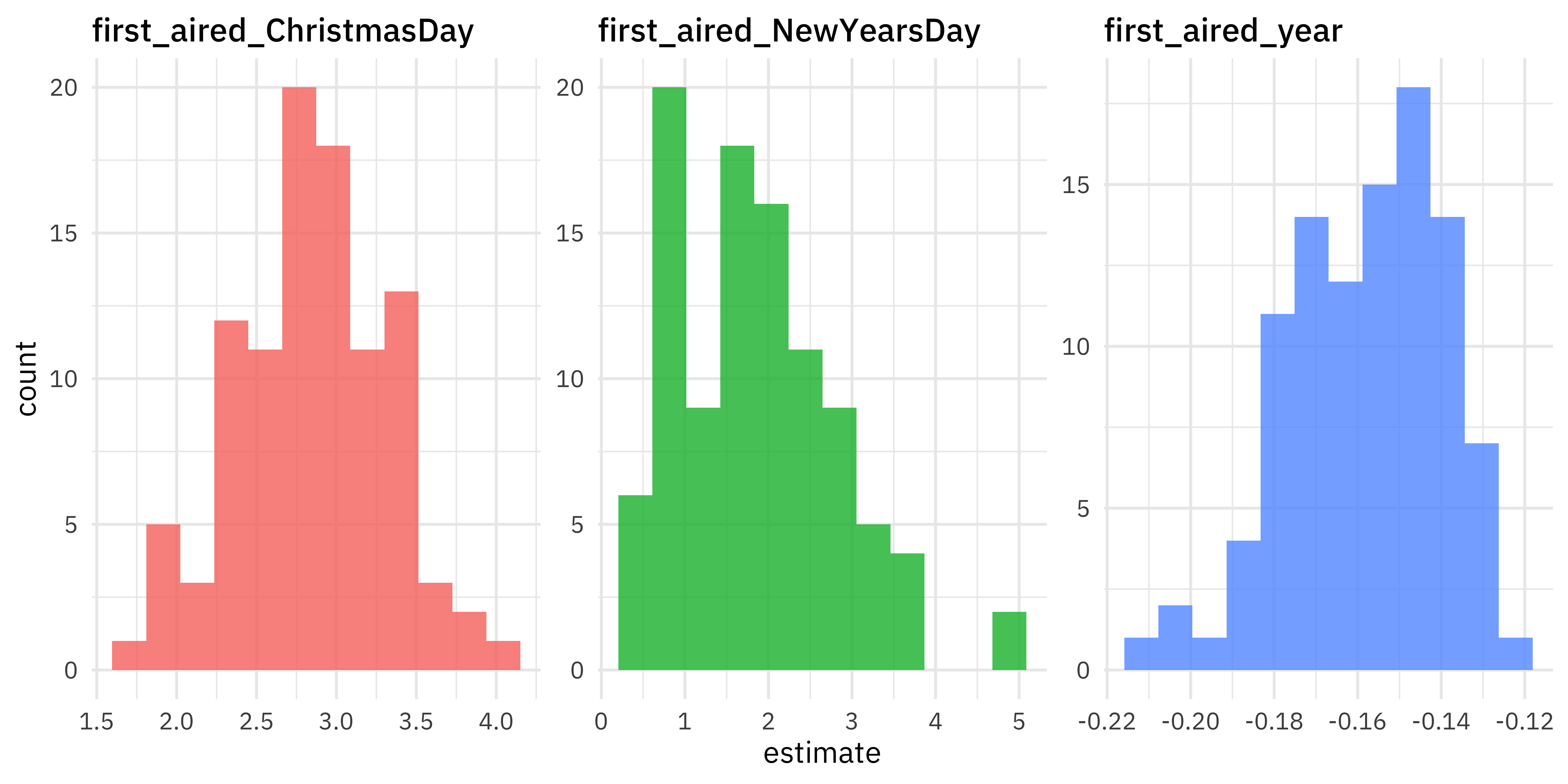
It looks like episodes airing on Christmas Day have much higher viewership, 2.5 to 3 million viewers higher than other days. Airing on New Years also looks like it is associated with more viewers, and we see evidence for a modest decrease in viewers with year.
- Posted on:
- November 27, 2021
- Length:
- 5 minute read, 1064 words
- Categories:
- rstats tidymodels
- Tags:
- rstats tidymodels