Predict #TidyTuesday giant pumpkin weights with workflowsets

This is the latest in my series of screencasts demonstrating how to use the tidymodels packages. If you are a tidymodels user, either just starting out or someone who has used the packages a lot, we are interested in your feedback on our priorities for 2022. The survey we fielded last year turned out to be very helpful in making decisions, so we would so appreciate your input again!

Today’s screencast is great for someone just starting out with workflowsets, the tidymodels package for handling multiple preprocessing/modeling combinations at once, with this week’s #TidyTuesday dataset on giant pumpkins from competitons. 🥧

Here is the code I used in the video, for those who prefer reading instead of or in addition to video.

Explore data

Our modeling goal is to predict the weight of giant pumpkins from other characteristics measured during a competition.

library(tidyverse)

pumpkins_raw <- readr::read_csv("https://raw.githubusercontent.com/rfordatascience/tidytuesday/master/data/2021/2021-10-19/pumpkins.csv")

pumpkins <-
  pumpkins_raw %>%
  separate(id, into = c("year", "type")) %>%
  mutate(across(c(year, weight_lbs, ott, place), parse_number)) %>%
  filter(type == "P") %>%
  select(weight_lbs, year, place, ott, gpc_site, country)

pumpkins

## # A tibble: 15,965 × 6
##    weight_lbs  year place   ott gpc_site                             country    
##         <dbl> <dbl> <dbl> <dbl> <chr>                                <chr>      
##  1      2032   2013     1   475 Uesugi Farms Weigh-off               United Sta…
##  2      1985   2013     2   453 Safeway World Championship Pumpkin … United Sta…
##  3      1894   2013     3   445 Safeway World Championship Pumpkin … United Sta…
##  4      1874.  2013     4   436 Elk Grove Giant Pumpkin Festival     United Sta…
##  5      1813   2013     5   430 The Great Howard Dill Giant Pumpkin… Canada     
##  6      1791   2013     6   431 Elk Grove Giant Pumpkin Festival     United Sta…
##  7      1784   2013     7   445 Uesugi Farms Weigh-off               United Sta…
##  8      1784.  2013     8   434 Stillwater Harvestfest               United Sta…
##  9      1780.  2013     9   422 Stillwater Harvestfest               United Sta…
## 10      1766.  2013    10   425 Durham Fair Weigh-Off                United Sta…
## # … with 15,955 more rows

The main relationship here is between the volume/size of the pumpkin (measured via “over-the-top inches”) and weight.

pumpkins %>%
  filter(ott > 20, ott < 1e3) %>%
  ggplot(aes(ott, weight_lbs, color = place)) +
  geom_point(alpha = 0.2, size = 1.1) +
  labs(x = "over-the-top inches", y = "weight (lbs)") +
  scale_color_viridis_c()

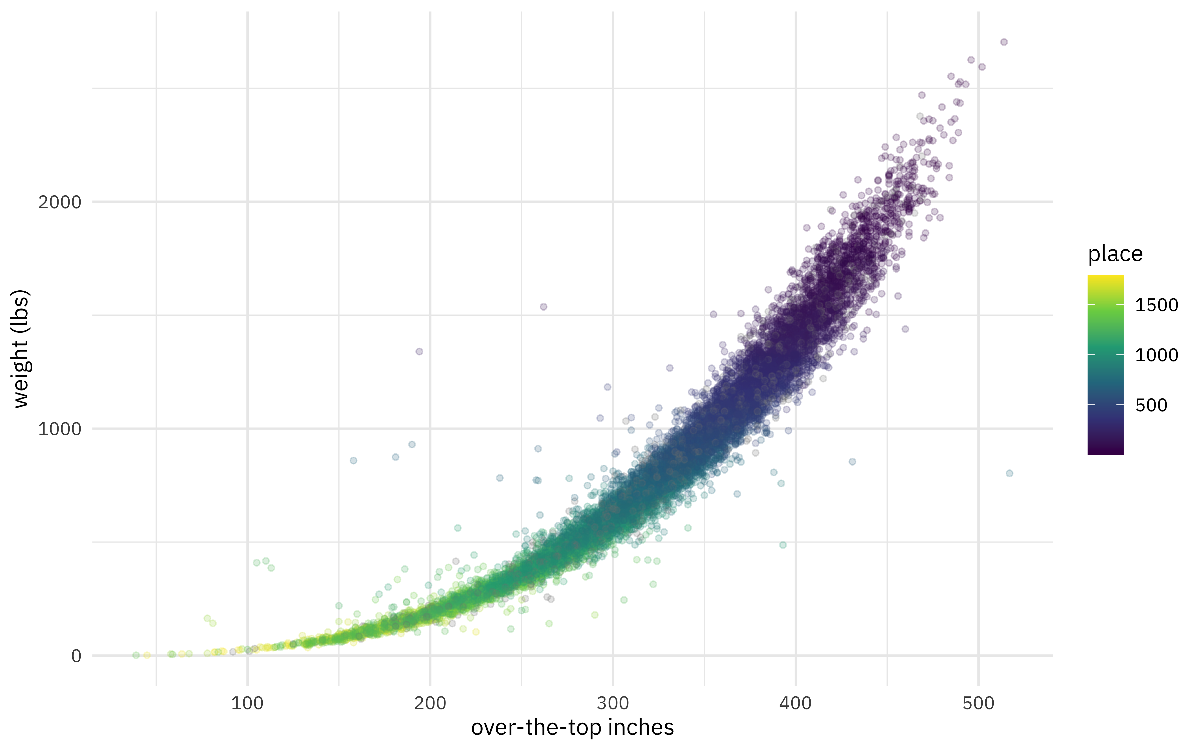
Big, heavy pumpkins placed closer to winning at the competitions, naturally!

Has there been any shift in this relationship over time?

pumpkins %>%
  filter(ott > 20, ott < 1e3) %>%
  ggplot(aes(ott, weight_lbs)) +
  geom_point(alpha = 0.2, size = 1.1, color = "gray60") +
  geom_smooth(aes(color = factor(year)),
    method = lm, formula = y ~ splines::bs(x, 3),
    se = FALSE, size = 1.5, alpha = 0.6
  ) +
  labs(x = "over-the-top inches", y = "weight (lbs)", color = NULL) +
  scale_color_viridis_d()

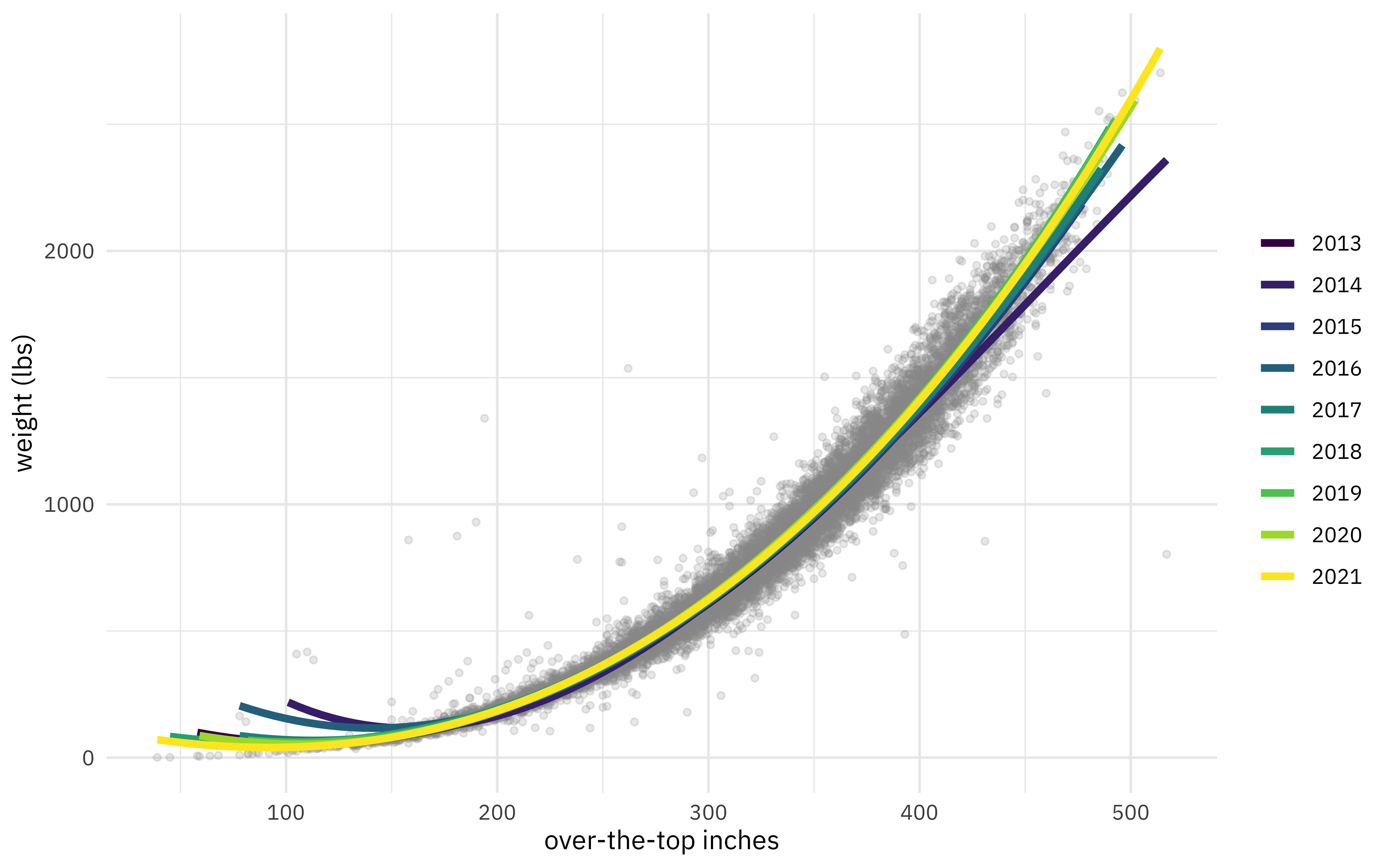
Hard to say, I think.

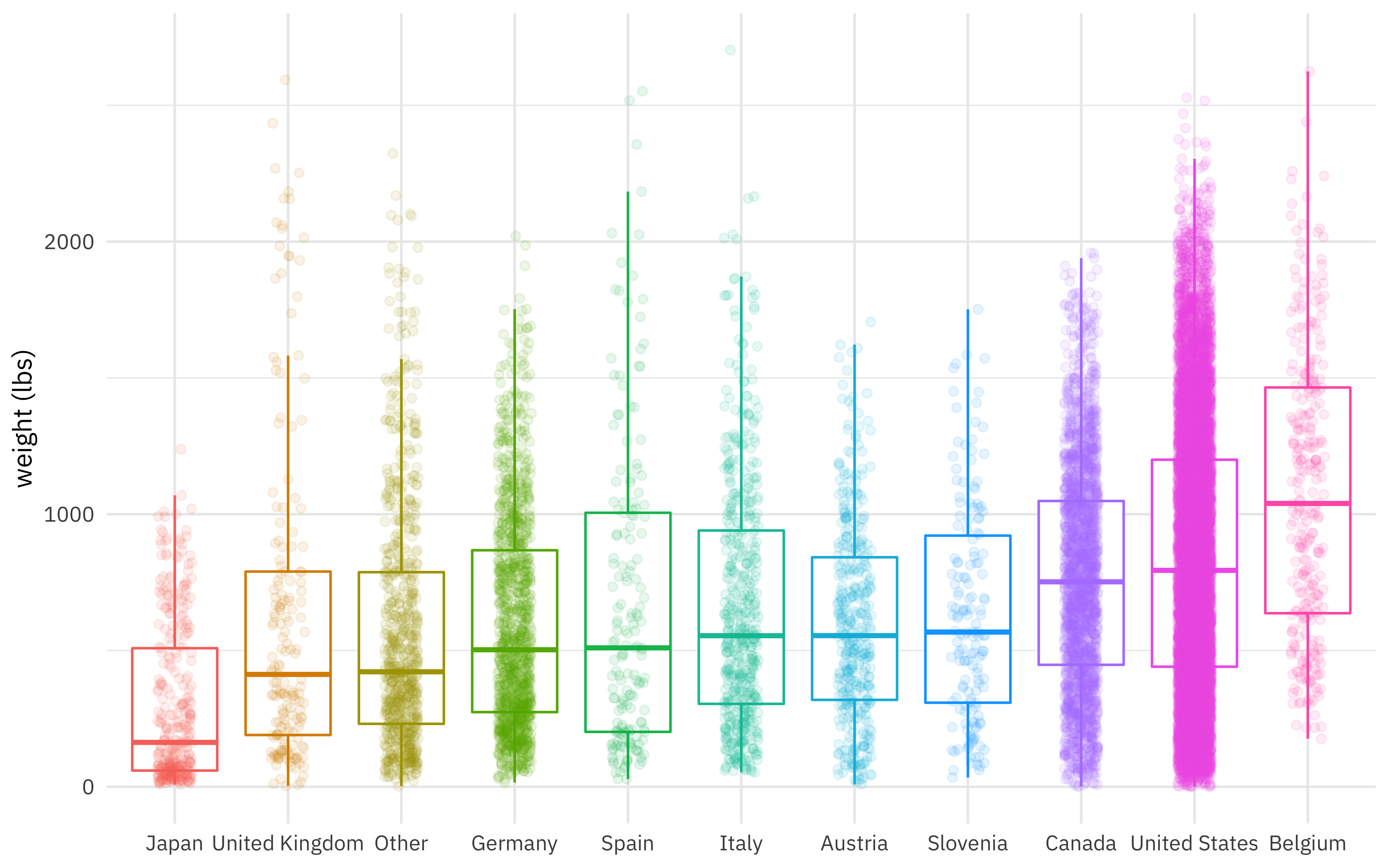
Which countries produced more or less massive pumpkins?

pumpkins %>%
  mutate(
    country = fct_lump(country, n = 10),
    country = fct_reorder(country, weight_lbs)
  ) %>%
  ggplot(aes(country, weight_lbs, color = country)) +
  geom_boxplot(outlier.colour = NA) +
  geom_jitter(alpha = 0.1, width = 0.15) +
  labs(x = NULL, y = "weight (lbs)") +
  theme(legend.position = "none")

Build and fit a workflow set

Let’s start our modeling by setting up our “data budget.” We’ll stratify by our outcome weight_lbs.

library(tidymodels)

set.seed(123)
pumpkin_split <- pumpkins %>%
  filter(ott > 20, ott < 1e3) %>%
  initial_split(strata = weight_lbs)

pumpkin_train <- training(pumpkin_split)
pumpkin_test <- testing(pumpkin_split)

set.seed(234)
pumpkin_folds <- vfold_cv(pumpkin_train, strata = weight_lbs)
pumpkin_folds

## #  10-fold cross-validation using stratification 
## # A tibble: 10 × 2
##    splits             id    
##    <list>             <chr> 
##  1 <split [8954/996]> Fold01
##  2 <split [8954/996]> Fold02
##  3 <split [8954/996]> Fold03
##  4 <split [8954/996]> Fold04
##  5 <split [8954/996]> Fold05
##  6 <split [8954/996]> Fold06
##  7 <split [8955/995]> Fold07
##  8 <split [8956/994]> Fold08
##  9 <split [8957/993]> Fold09
## 10 <split [8958/992]> Fold10

Next, let’s create three data preprocessing recipes: one that only pools infrequently used factors levels, one that also creates indicator variables, and finally one that also creates spline terms for over-the-top inches.

base_rec <-
  recipe(weight_lbs ~ ott + year + country + gpc_site,
    data = pumpkin_train
  ) %>%
  step_other(country, gpc_site, threshold = 0.02)

ind_rec <-
  base_rec %>%
  step_dummy(all_nominal_predictors())

spline_rec <-
  ind_rec %>%
  step_bs(ott)

Then, let’s create three model specifications: a random forest model, a MARS model, and a linear model.

rf_spec <-
  rand_forest(trees = 1e3) %>%
  set_mode("regression") %>%
  set_engine("ranger")

mars_spec <-
  mars() %>%
  set_mode("regression") %>%
  set_engine("earth")

lm_spec <- linear_reg()

Now it’s time to put the preprocessing and models together in a workflow_set().

pumpkin_set <-
  workflow_set(
    list(base_rec, ind_rec, spline_rec),
    list(rf_spec, mars_spec, lm_spec),
    cross = FALSE
  )

pumpkin_set

## # A workflow set/tibble: 3 × 4
##   wflow_id             info             option    result    
##   <chr>                <list>           <list>    <list>    
## 1 recipe_1_rand_forest <tibble [1 × 4]> <opts[0]> <list [0]>
## 2 recipe_2_mars        <tibble [1 × 4]> <opts[0]> <list [0]>
## 3 recipe_3_linear_reg  <tibble [1 × 4]> <opts[0]> <list [0]>

We use cross = FALSE because we don’t want every combination of these components, only three options to try. Let’s fit these possible candidates to our resamples to see which one performs best.

doParallel::registerDoParallel()
set.seed(2021)

pumpkin_rs <-
  workflow_map(
    pumpkin_set,
    "fit_resamples",
    resamples = pumpkin_folds
  )

pumpkin_rs

## # A workflow set/tibble: 3 × 4
##   wflow_id             info             option    result   
##   <chr>                <list>           <list>    <list>   
## 1 recipe_1_rand_forest <tibble [1 × 4]> <opts[1]> <rsmp[+]>
## 2 recipe_2_mars        <tibble [1 × 4]> <opts[1]> <rsmp[+]>
## 3 recipe_3_linear_reg  <tibble [1 × 4]> <opts[1]> <rsmp[+]>

Evaluate workflow set

How did our three candidates do?

autoplot(pumpkin_rs)

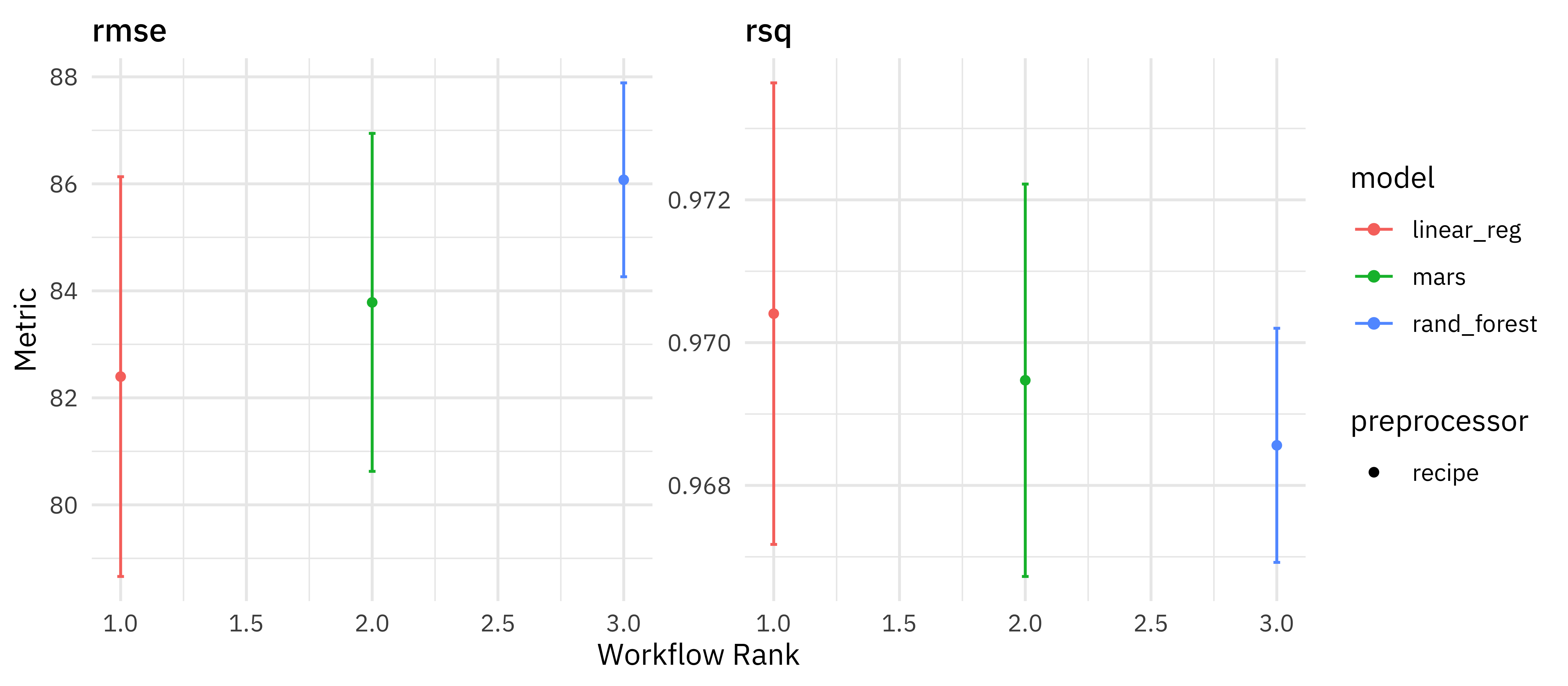
There is not much difference between the three options, and if anything, our linear model with spline feature engineering maybe did better. This is nice because it’s a simpler model!

collect_metrics(pumpkin_rs)

## # A tibble: 6 × 9
##   wflow_id    .config     preproc model  .metric .estimator   mean     n std_err
##   <chr>       <chr>       <chr>   <chr>  <chr>   <chr>       <dbl> <int>   <dbl>
## 1 recipe_1_r… Preprocess… recipe  rand_… rmse    standard   86.1      10 1.10e+0
## 2 recipe_1_r… Preprocess… recipe  rand_… rsq     standard    0.969    10 9.97e-4
## 3 recipe_2_m… Preprocess… recipe  mars   rmse    standard   83.8      10 1.92e+0
## 4 recipe_2_m… Preprocess… recipe  mars   rsq     standard    0.969    10 1.67e-3
## 5 recipe_3_l… Preprocess… recipe  linea… rmse    standard   82.4      10 2.27e+0
## 6 recipe_3_l… Preprocess… recipe  linea… rsq     standard    0.970    10 1.97e-3

We can extract the workflow we want to use and fit it to our training data.

final_fit <-
  extract_workflow(pumpkin_rs, "recipe_3_linear_reg") %>%
  fit(pumpkin_train)

We can use an object like this to predict, such as on the test data like predict(final_fit, pumpkin_test), or we can examine the model parameters.

tidy(final_fit) %>%
  arrange(-abs(estimate))

## # A tibble: 15 × 5
##    term                                   estimate std.error statistic   p.value
##    <chr>                                     <dbl>     <dbl>     <dbl>     <dbl>
##  1 (Intercept)                            -9731.     675.      -14.4   1.30e- 46
##  2 ott_bs_3                                2585.      25.6     101.    0        
##  3 ott_bs_2                                 450.      11.9      37.9   2.75e-293
##  4 ott_bs_1                                -345.      36.3      -9.50  2.49e- 21
##  5 gpc_site_Ohio.Valley.Giant.Pumpkin.Gr…    21.1      7.80      2.70  6.89e-  3
##  6 country_United.States                     11.9      5.66      2.11  3.53e-  2
##  7 gpc_site_Stillwater.Harvestfest           11.6      7.87      1.48  1.40e-  1
##  8 country_Germany                          -11.5      6.68     -1.71  8.64e-  2
##  9 country_other                            -10.7      6.33     -1.69  9.13e-  2
## 10 country_Canada                             9.29     6.12      1.52  1.29e-  1
## 11 country_Italy                              8.12     7.02      1.16  2.47e-  1
## 12 gpc_site_Elk.Grove.Giant.Pumpkin.Fest…    -7.81     7.70     -1.01  3.10e-  1
## 13 year                                       4.89     0.334    14.6   5.03e- 48
## 14 gpc_site_Wiegemeisterschaft.Berlin.Br…     1.51     8.07      0.187 8.51e-  1
## 15 gpc_site_other                             1.41     5.60      0.251 8.02e-  1

The spline terms are by far the most important, but we do see evidence of certain sites and countries being predictive of weight (either up or down) as well as a small trend of heavier pumpkins with year.

Don’t forget to take the tidymodels survey for 2022 priorities!