tidytext 0.1.6

I am pleased to announce that tidytext 0.1.6 is now on CRAN!

Most of this release, as well as the 0.1.5 release which I did not blog about, was for maintenance, updates to align with API changes from tidytext’s dependencies, and bugs. I just spent a good chunk of effort getting tidytext to pass R CMD check on older versions of R despite the fact that some of the packages in tidytext’s Suggests require recent versions of R. FUN TIMES. I was glad to get it working, though, because I know that we have users, some teaching on university campuses, etc, who are constrained to older versions of R in various environments.

There are some more interesting updates. For example, did you know about the new-ish stopwords package? This package provides access to stopword lists from multiple sources in multiple languages. If you would like to access these in a list data structure, go to the original package. But if you like your text tidy, I GOT YOU.

library(tidytext)

get_stopwords()

## # A tibble: 175 x 2
##    word      lexicon 
##    <chr>     <chr>   
##  1 i         snowball
##  2 me        snowball
##  3 my        snowball
##  4 myself    snowball
##  5 we        snowball
##  6 our       snowball
##  7 ours      snowball
##  8 ourselves snowball
##  9 you       snowball
## 10 your      snowball
## # ... with 165 more rows

get_stopwords(source = "smart")

## # A tibble: 571 x 2
##    word        lexicon
##    <chr>       <chr>  
##  1 a           smart  
##  2 a's         smart  
##  3 able        smart  
##  4 about       smart  
##  5 above       smart  
##  6 according   smart  
##  7 accordingly smart  
##  8 across      smart  
##  9 actually    smart  
## 10 after       smart  
## # ... with 561 more rows

get_stopwords(language = "ru")

## # A tibble: 159 x 2
##    word  lexicon 
##    <chr> <chr>   
##  1 и     snowball
##  2 в     snowball
##  3 во    snowball
##  4 не    snowball
##  5 что   snowball
##  6 он    snowball
##  7 на    snowball
##  8 я     snowball
##  9 с     snowball
## 10 со    snowball
## # ... with 149 more rows

get_stopwords(language = "it")

## # A tibble: 279 x 2
##    word  lexicon 
##    <chr> <chr>   
##  1 ad    snowball
##  2 al    snowball
##  3 allo  snowball
##  4 ai    snowball
##  5 agli  snowball
##  6 all   snowball
##  7 agl   snowball
##  8 alla  snowball
##  9 alle  snowball
## 10 con   snowball
## # ... with 269 more rows

This allows users to implement text mining tasks using tidy data principles that have been difficult before now. What if we would like to find the most common words in, say, Rainer Maria Rilke’s work, but in the original German?

library(gutenbergr)
library(tidyverse)

raw_rilke <- gutenberg_download(c(24288, 33863, 2188, 34521),
                                meta_fields = "title") %>%
    mutate(text = iconv(text, from = "latin-9", to = "UTF-8"))

tidy_rilke <- raw_rilke %>%
    unnest_tokens(word, text) %>%
    count(title, word, sort = TRUE) %>%
    anti_join(get_stopwords(language = "de"))

tidy_rilke

## # A tibble: 18,698 x 3
##    title                                       word       n
##    <chr>                                       <chr>  <int>
##  1 Die Aufzeichnungen des Malte Laurids Brigge immer    160
##  2 Die Aufzeichnungen des Malte Laurids Brigge ganz     155
##  3 Die Aufzeichnungen des Malte Laurids Brigge mehr     140
##  4 Die Aufzeichnungen des Malte Laurids Brigge konnte   132
##  5 Die Aufzeichnungen des Malte Laurids Brigge kam      123
##  6 Die Aufzeichnungen des Malte Laurids Brigge zeit     120
##  7 Die Aufzeichnungen des Malte Laurids Brigge schon    119
##  8 Die Aufzeichnungen des Malte Laurids Brigge sah      101
##  9 Die Aufzeichnungen des Malte Laurids Brigge hätte     97
## 10 Die Aufzeichnungen des Malte Laurids Brigge wäre      95
## # ... with 18,688 more rows

tidy_rilke %>%
    group_by(title) %>%
    top_n(12) %>%
    ungroup %>%
    mutate(word = reorder(word, n),
           title = factor(title,
                          levels = c("Das Stunden-Buch",
                                     "Das Buch der Bilder",
                                     "Neue Gedichte",
                                     "Die Aufzeichnungen des Malte Laurids Brigge"))) %>%
    group_by(title, word) %>%    
    arrange(desc(n)) %>%  
    ungroup() %>%
    mutate(word = factor(paste(word, title, sep = "__"), 
                         levels = rev(paste(word, title, sep = "__")))) %>%
    ggplot(aes(word, n, fill = title)) +
    geom_col(alpha = 0.8, show.legend = FALSE) +
    coord_flip() +
    facet_wrap(~title, scales = "free") +
    scale_y_continuous(expand = c(0,0)) +
    scale_x_discrete(labels = function(x) gsub("__.+$", "", x)) +
    labs(x = NULL, y = "Number of uses in each book",
         title = "Word use in the poetry of Rainer Maria Rilke",
         subtitle = "The most common words after stopword removal")

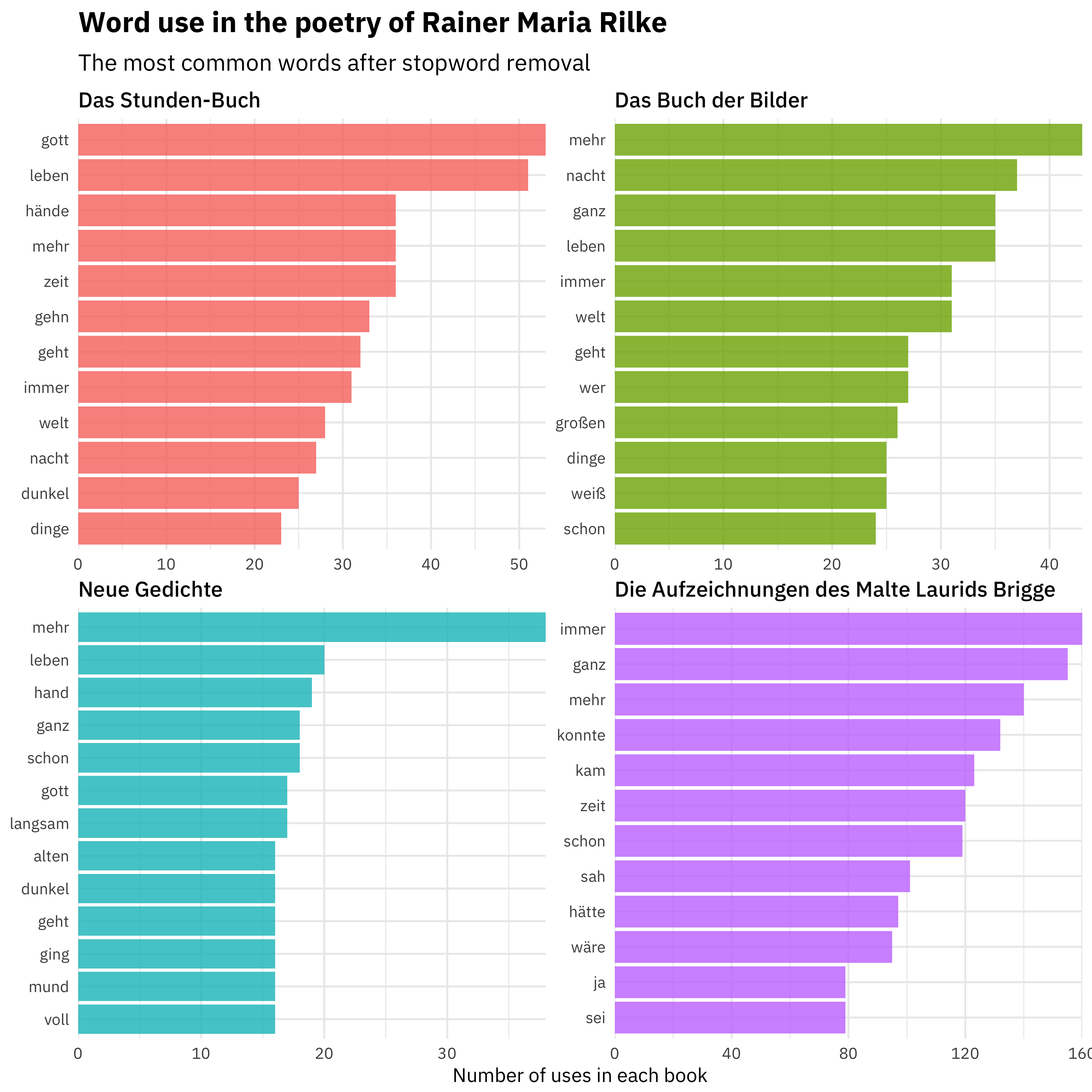
The first three works here are poetry (The Book of Hours, The Book of Images, and New Poems) while the last is a book of prose (The Notebooks of Malte Laurids Brigge). We can see the different themes and word use here, even just by counting up word frequencies. Now, if I actually spoke German fluently, I know this would mean more to me, but even to my English-speaking eyes, we can see meaningful trends. These are all still quite common words (the Snowball stopword lists are not terribly large) but some of these works are more religious (God, life) and some more focused on narrating events, and so forth.

Another addition in this release is a dataset of negators, modals, and adverbs (only in English). These are words that can affect sentiment analysis, either by intensifying words or negating them.

nma_words %>%
    count(modifier)

## # A tibble: 3 x 2
##   modifier     n
##   <chr>    <int>
## 1 adverb      22
## 2 modal        7
## 3 negator     15

You can read more from Saif Mohammad about how these kinds of words can affect sentiment analysis. One of the reasons that tidy data principles are so well suited to text mining is that you can interrogate sentiment scores and get at questions like these quite naturally. I talk about this in my DataCamp course, and also you can read about this in our book, in the chapter on n-grams and the case study on Usenet messages.

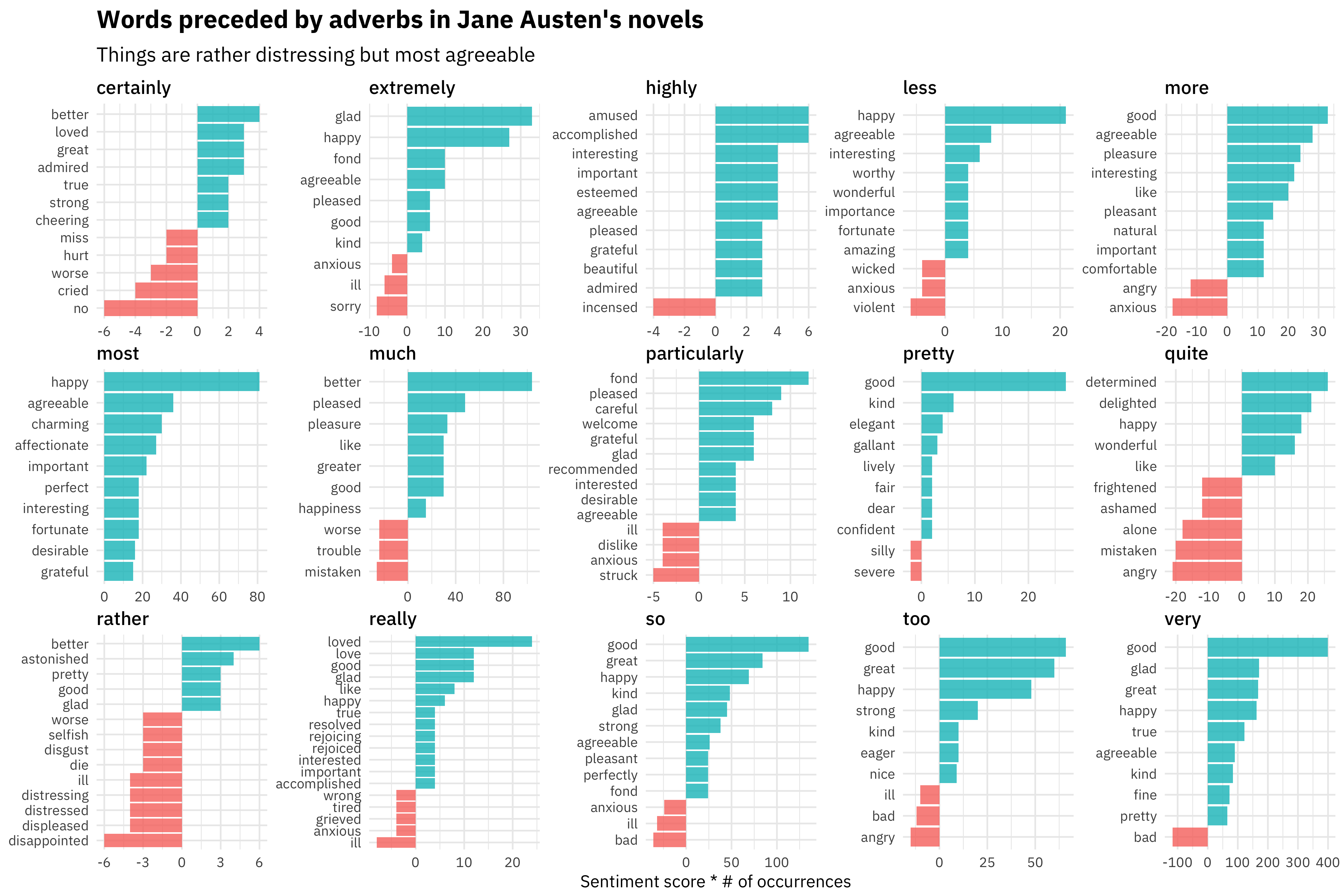
For example, we can ask which words in Jane Austen’s novels are more likely to appear after these adverbs?

library(janeaustenr)

adverbs <- nma_words %>%
    filter(modifier == "adverb") %>%
    pull(word)

austen_bigrams <- austen_books() %>%
    unnest_tokens(bigram, text, token = "ngrams", n = 2) %>%
    count(bigram, sort = TRUE) %>%
    separate(bigram, c("word1", "word2"), sep = " ")

austen_bigrams %>%
    filter(word1 %in% adverbs) %>%
    count(word1, word2, wt = n, sort = TRUE) %>%
    inner_join(get_sentiments("afinn"), by = c(word2 = "word")) %>%
    mutate(contribution = score * nn) %>%
    group_by(word1) %>%
    filter(n() > 10) %>%
    top_n(10, abs(contribution)) %>%
    ungroup() %>%
    mutate(word2 = reorder(paste(word2, word1, sep = "__"), contribution)) %>%
    ggplot(aes(word2, contribution, fill = contribution > 0)) +
    geom_col(alpha = 0.8, show.legend = FALSE) +
    facet_wrap(~ word1, scales = "free", nrow = 3) +
    scale_x_discrete(labels = function(x) gsub("__.+$", "", x)) +
    coord_flip() +
    labs(x = NULL, y = "Sentiment score * # of occurrences",
         title = "Words preceded by adverbs in Jane Austen's novels",
         subtitle = "Things are rather distressing but most agreeable")

Gosh, I love this A LOT because you can see really common Jane Austen word patterns here. Some people are extremely agreeable, but sometimes you can’t help but be highly incensed. I am particularly fond of this kind of text mining.

To see any more details of how to use tidytext functions, you can check out the documentation, vignettes, and news for tidytext at our package website. Let me know if you have questions!