tidytext 0.1.3
By Julia Silge
June 18, 2017
I am pleased to announce that tidytext 0.1.3 is now on CRAN!
In this release, my collaborator David Robinson and I have fixed a handful of bugs, added tidiers for LDA models from the mallet package, and updated functions for changes to quanteda’s API. You can check out the NEWS for more details on changes.
One enhancement in this release is the addition of the Loughran and McDonald sentiment lexicon of words specific to financial reporting. Sentiment lexicons are lists of words that are used to assess the emotion or opinion content of text by adding up the sentiment scores of individual words within that text; the tidytext package contains three general purpose English sentiment lexicons. The positive or negative meaning of a word can depend on its context, though. A word like “risk” has a negative meaning in most general contexts but may be more neutral for financial reporting. Context-specific sentiment lexicons like the Loughran-McDonald dictionary provide a way to deal with this.
This financial lexicon labels words with six possible sentiments.
library(tidytext)
library(tidyverse)

get_sentiments("loughran") %>%
    count(sentiment, sort = TRUE)
## # A tibble: 6 x 2
## sentiment n
## <chr> <int>
## 1 negative 2355
## 2 litigious 903
## 3 positive 354
## 4 uncertainty 297
## 5 constraining 184
## 6 superfluous 56An example
I recently saw a sentiment analysis by Michael Toth of Warren Buffett’s letters to shareholders. It’s a super interesting analysis, done well, but we can see from some of the plots in that analysis that the specifically financial nature of these documents would make a financial sentiment lexicon a great choice. Let’s scrape the letters from Berkshire Hathaway, Warren Buffett’s company, and then implement a sentiment analysis using this new lexicon.
library(rvest)
library(pdftools)

urls_oldest <- paste0("http://www.berkshirehathaway.com/letters/",
                     seq(1977, 1997), ".html")
html_urls <- c(urls_oldest,
               "http://www.berkshirehathaway.com/letters/1998htm.html",
               "http://www.berkshirehathaway.com/letters/1999htm.html",
               "http://www.berkshirehathaway.com/2000ar/2000letter.html",
               "http://www.berkshirehathaway.com/2001ar/2001letter.html")

letters_html <- html_urls %>%
    map_chr(~ read_html(.) %>%
                html_text())

urls_newest <- paste0("http://www.berkshirehathaway.com/letters/",
                      seq(2003, 2016), "ltr.pdf")

pdf_urls <- c("http://www.berkshirehathaway.com/letters/2002pdf.pdf",
              urls_newest)

letters_pdf <- pdf_urls %>%
    map_chr(~ pdf_text(.) %>% paste(collapse = " "))

letters <- data_frame(year = seq(1977, 2016),
                      text = c(letters_html, letters_pdf))
Now we have the letters, and can convert this to a tidy text format.
tidy_letters <- letters %>%
    unnest_tokens(word, text) %>%
    add_count(year) %>%
    rename(year_total = n)

tidy_letters
## # A tibble: 486,560 x 3
## year word year_total
## <int> <chr> <int>
## 1 1977 chairman's 3063
## 2 1977 letter 3063
## 3 1977 1977 3063
## 4 1977 berkshire 3063
## 5 1977 hathaway 3063
## 6 1977 inc 3063
## 7 1977 to 3063
## 8 1977 the 3063
## 9 1977 stockholders 3063
## 10 1977 of 3063
## # ... with 486,550 more rowsNext, let’s implement the sentiment analysis.
letter_sentiment <- tidy_letters %>%
    inner_join(get_sentiments("loughran"))

letter_sentiment
## # A tibble: 20,921 x 4
## year word year_total sentiment
## <int> <chr> <int> <chr>
## 1 1977 better 3063 positive
## 2 1977 anticipated 3063 uncertainty
## 3 1977 gains 3063 positive
## 4 1977 gains 3063 positive
## 5 1977 losses 3063 negative
## 6 1977 gains 3063 positive
## 7 1977 losses 3063 negative
## 8 1977 anticipated 3063 uncertainty
## 9 1977 indemnity 3063 litigious
## 10 1977 better 3063 positive
## # ... with 20,911 more rowsNow we have all we need to see the relative changes in these sentiments over the years.
letter_sentiment %>%
    count(year, year_total, sentiment) %>%
    filter(sentiment %in% c("positive", "negative",
                            "uncertainty", "litigious")) %>%
    mutate(sentiment = factor(sentiment, levels = c("negative",
                                                    "positive",
                                                    "uncertainty",
                                                    "litigious"))) %>%
    ggplot(aes(year, n / year_total, fill = sentiment)) +
    geom_area(position = "identity", alpha = 0.5) +
    labs(y = "Relative frequency", x = NULL,
         title = "Sentiment analysis of Warren Buffett's shareholder letters",
         subtitle = "Using the Loughran-McDonald lexicon")
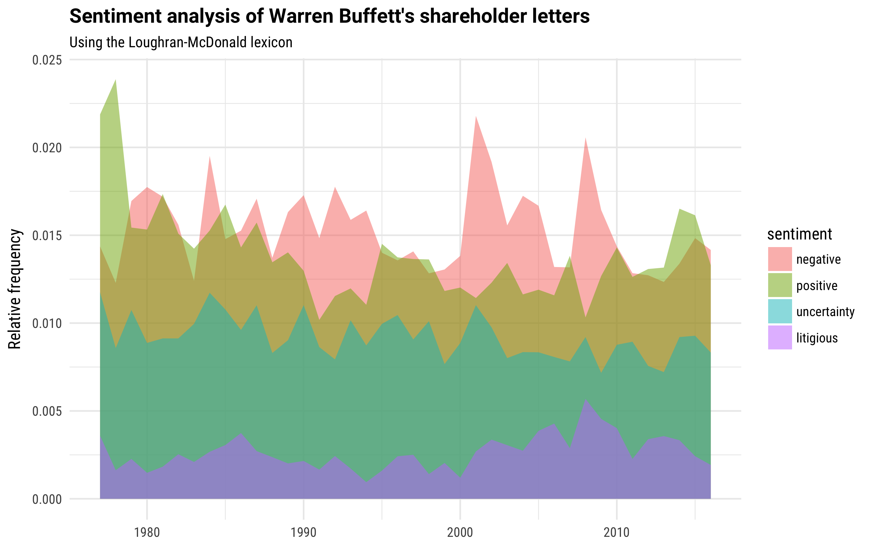
We see negative sentiment spiking, higher than positive sentiment, during the financial upheaval of 2008, the collapse of the dot-com bubble in the early 2000s, and the recession of the 1990s. Overall, though, notice that the balance of positive to negative sentiment is not as skewed to positive as when you use one of the general purpose sentiment lexicons.
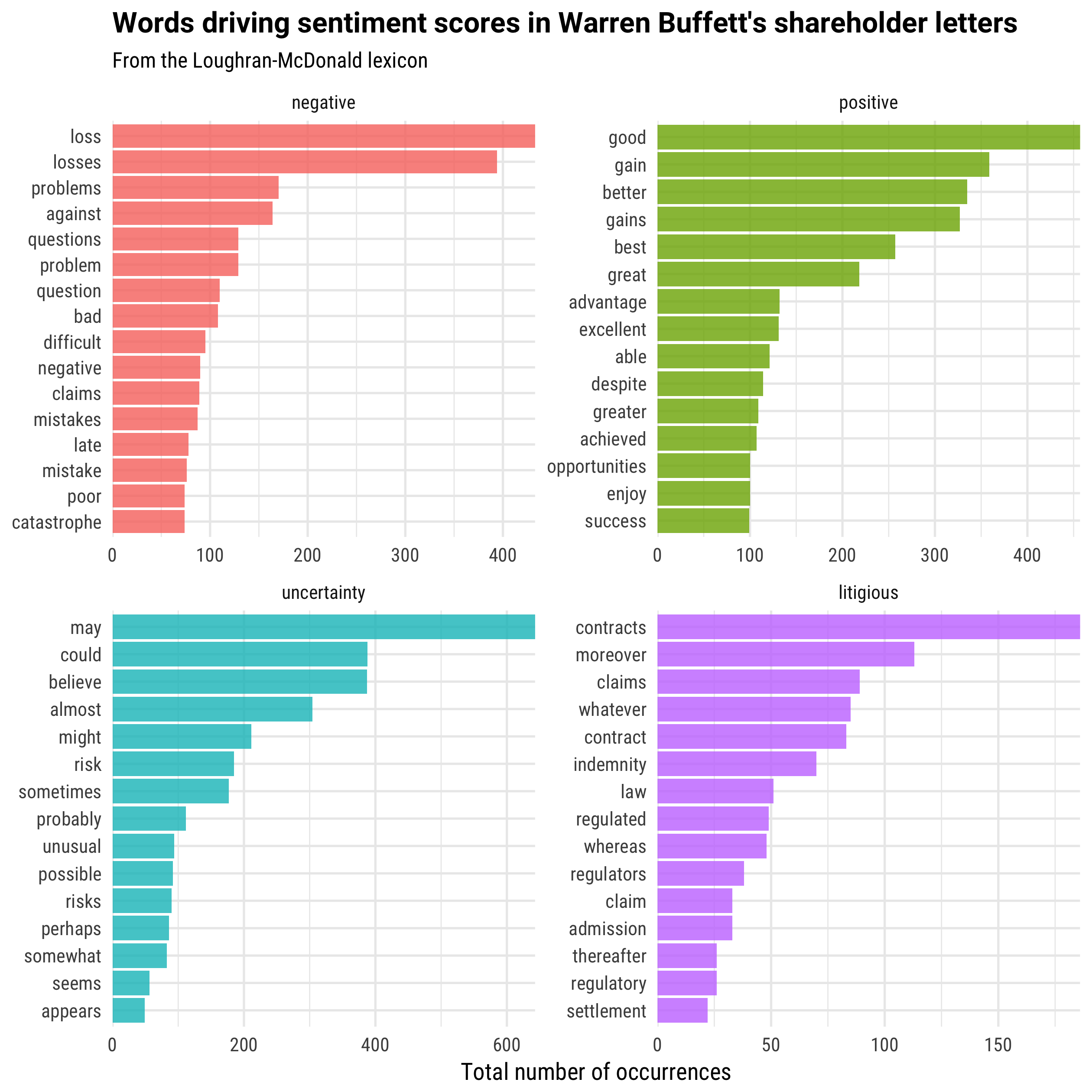
This happens because of the words that are driving the sentiment score in these different cases. When using the financial sentiment lexicon, the words have specifically been chosen for a financial context. What words are driving these sentiment scores?
letter_sentiment %>%
    count(sentiment, word) %>%
    filter(sentiment %in% c("positive", "negative",
                            "uncertainty", "litigious")) %>%
    group_by(sentiment) %>%
    top_n(15) %>%
    ungroup %>%
    mutate(word = reorder(word, n)) %>%
    mutate(sentiment = factor(sentiment, levels = c("negative",
                                                    "positive",
                                                    "uncertainty",
                                                    "litigious"))) %>%
    ggplot(aes(word, n, fill = sentiment)) +
    geom_col(alpha = 0.8, show.legend = FALSE) +
    coord_flip() +
    scale_y_continuous(expand = c(0,0)) +
    facet_wrap(~sentiment, scales = "free") +
    labs(x = NULL, y = "Total number of occurrences",
         title = "Words driving sentiment scores in Warren Buffett's shareholder letters",
         subtitle = "From the Loughran-McDonald lexicon")
The End
Checking which words are driving a sentiment score is not only important when dealing with financial text, but all text; using tidy data principles makes it possible and not too difficult to dig into such an analysis. Our upcoming book Text Mining with R explores how applying tidy data principles to this and lots of other text mining tasks makes your time and energy well spent. In the meantime, get the new version of tidytext and let us know on GitHub if you run into any issues!