Scraping CRAN with rvest

I am one of the organizers for a session at userR 2017 this coming July that will focus on discovering and learning about R packages. How do R users find packages that meet their needs? Can we make this process easier? As somebody who is relatively new to the R world compared to many, this is a topic that resonates with me and I am happy to be part of the discussion. I am working on this session with John Nash and Spencer Graves, and we hope that some useful discussion and results come out of the session.

In preparation for this session, I wanted to look at the distribution of R packages by date, number of version, etc. There have been some great plots that came out around the time when CRAN passed the 10,000 package mark but most of the code to make those scripts involve packages and idioms I am less familiar with, so here is an rvest and tidyverse centered version of those analyses!

Scraping CRAN

The first thing we need to do is get all the packages that are currently available on CRAN. Let’s use rvest to scrape the page that lists all the packages currently on CRAN. It also has some other directories besides packages so we can use filter to remove the things that don’t look like R packages.

library(rvest)
library(stringr)
library(lubridate)
library(tidyverse)

cran_link <- function(...) {
    file.path("https://cran.rstudio.com/src/contrib", ...)
}

pkgs_raw <- read_html(cran_link()) %>% 
    html_nodes("table") %>% 
    .[[1]] %>%
    html_table()

pkgs_raw <- pkgs_raw[,-1]

pkgs <- pkgs_raw %>%
    filter(Size != "-",
           str_detect(Name, "tar.gz$")) %>%
    mutate(Date = dmy_hm(`Last modified`),
           Name = str_extract(Name, "^[^_]+(?=_)")) %>%
    select(-Size, -Description) %>%
    as_tibble()

pkgs

## # A tibble: 10,211 × 3
##            Name   `Last modified`                Date
##           <chr>             <chr>              <dttm>
## 1            A3 16-Aug-2015 21:05 2015-08-16 21:05:00
## 2       ABC.RAP 20-Oct-2016 08:52 2016-10-20 08:52:00
## 3   ABCanalysis 23-Aug-2016 12:57 2016-08-23 12:57:00
## 4      ABCoptim 17-Nov-2016 09:04 2016-11-17 09:04:00
## 5         ABCp2 04-Feb-2016 10:27 2016-02-04 10:27:00
## 6  ABHgenotypeR 04-Feb-2016 10:27 2016-02-04 10:27:00
## 7           ACA 10-Mar-2016 16:55 2016-03-10 16:55:00
## 8        ACCLMA 29-Oct-2012 12:13 2012-10-29 12:13:00
## 9           ACD 31-Oct-2013 19:59 2013-10-31 19:59:00
## 10         ACDm 16-Jul-2016 10:19 2016-07-16 10:19:00
## # ... with 10,201 more rows

So that’s currently available packages!

Now let’s turn to the archive. Let’s do a similar operation.

archives_raw <- read_html(cran_link("Archive")) %>% 
    html_nodes("table") %>% 
    .[[1]] %>%
    html_table()

archives_raw <- archives_raw[,-1]

archives_processed <- archives_raw %>%
    filter(str_detect(Name, "/$")) %>%
    mutate(Date = dmy_hm(`Last modified`),
           Name = str_sub(Name, end = -2)) %>%
    select(-Size, -Description) %>%
    as_tibble()

archives_processed

## # A tibble: 8,897 × 3
##            Name   `Last modified`                Date
##           <chr>             <chr>              <dttm>
## 1            A3 16-Aug-2015 21:05 2015-08-16 21:05:00
## 2   ABCExtremes 19-Jun-2015 11:26 2015-06-19 11:26:00
## 3   ABCanalysis 23-Aug-2016 12:57 2016-08-23 12:57:00
## 4      ABCoptim 17-Nov-2016 09:04 2016-11-17 09:04:00
## 5         ABCp2 01-Jul-2015 06:12 2015-07-01 06:12:00
## 6  ABHgenotypeR 04-Feb-2016 10:27 2016-02-04 10:27:00
## 7           ACD 31-Oct-2013 19:59 2013-10-31 19:59:00
## 8          ACDm 16-Jul-2016 10:19 2016-07-16 10:19:00
## 9          ACEt 18-Nov-2016 21:19 2016-11-18 21:19:00
## 10         ACNE 27-Oct-2015 07:09 2015-10-27 07:09:00
## # ... with 8,887 more rows

That is good, but now we need to get more detailed information for packages that have been archived at least once to get the date they originally were released and how many versions they have had.

Visiting every page in the archive

Let’s set up a function for scraping an individual page for a package and apply that to every page in the archive. This step takes A WHILE because it queries a web page for every package in the CRAN archive. I’ve set this up with map from purrr; it is one of my favorite ways to organize tasks these days.

read_page <- function(name) {
    message(name)
    read_html(cran_link("Archive", name)) %>% 
        html_nodes("td") %>% 
        html_text()
}

archives_scraped <- archives_processed %>%
    mutate(page = map(Name, read_page))

What do these pages look like?

archives_scraped$page[8457]

## [[1]]
##  [1] ""                      "Parent Directory"      " "                     "  - "                 
##  [5] " "                     ""                      "tidytext_0.1.0.tar.gz" "28-Apr-2016 09:50  "  
##  [9] "1.4M"                  " "                     ""                      "tidytext_0.1.1.tar.gz"
## [13] "25-Jun-2016 17:07  "   "1.5M"                  " "

This is exactly what we need: the dates that the packages were released and how many times they have been released. Let’s use mutate and map again to extract these values.

archives <- archives_scraped %>%
    mutate(Date = dmy_hm(map_chr(page, ~ .[8])),
           ArchivedVersions = map_dbl(page, ~ length(.) / 5 - 1)) %>%
    select(-page)

archives

## # A tibble: 8,897 × 4
##            Name   `Last modified`                Date ArchivedVersions
##           <chr>             <chr>              <dttm>            <dbl>
## 1            A3 16-Aug-2015 21:05 2013-02-07 09:00:00                2
## 2   ABCExtremes 19-Jun-2015 11:26 2013-05-15 08:45:00                1
## 3   ABCanalysis 23-Aug-2016 12:57 2015-04-20 15:40:00                5
## 4      ABCoptim 17-Nov-2016 09:04 2013-11-05 17:00:00                2
## 5         ABCp2 01-Jul-2015 06:12 2013-04-10 15:04:00                2
## 6  ABHgenotypeR 04-Feb-2016 10:27 2016-01-21 07:26:00                1
## 7           ACD 31-Oct-2013 19:59 2012-11-27 06:43:00                2
## 8          ACDm 16-Jul-2016 10:19 2015-07-16 12:24:00                2
## 9          ACEt 18-Nov-2016 21:19 2016-02-14 17:48:00                7
## 10         ACNE 27-Oct-2015 07:09 2011-09-16 17:43:00                4
## # ... with 8,887 more rows

Putting it together

Now it’s time to join the data from the currently available packages and the archives.

• Packages that are in archives but not pkgs are no longer on CRAN.
• Packages that are in pkgs but not archives only have one CRAN release.
• Packages that are in both dataframes have had more than one CRAN release.

Sounds like a good time to use anti_join and inner_join.

all_pkgs <- bind_rows(archives %>% 
                          anti_join(pkgs, by = "Name") %>% 
                          mutate(Archived = TRUE),
                      pkgs %>% 
                          anti_join(archives, by = "Name") %>% 
                          mutate(ArchivedVersions = 0,
                                 Archived = FALSE),
                      archives %>%
                          semi_join(pkgs, by = "Name") %>%
                          mutate(Archived = FALSE)) %>%
    mutate(Versions = ifelse(Archived, ArchivedVersions, ArchivedVersions + 1)) %>%
    arrange(Name)

all_pkgs

## # A tibble: 11,489 × 6
##           Name   `Last modified`                Date ArchivedVersions Archived Versions
##          <chr>             <chr>              <dttm>            <dbl>    <lgl>    <dbl>
## 1           A3 16-Aug-2015 21:05 2013-02-07 09:00:00                2    FALSE        3
## 2         aaMI 30-Jul-2010 12:17 2005-06-24 15:55:00                2     TRUE        2
## 3       abbyyR 20-Jun-2016 15:32 2015-06-12 04:43:00                7    FALSE        8
## 4          abc 05-May-2015 09:34 2010-10-05 08:45:00               10    FALSE       11
## 5     abc.data 05-May-2015 09:34 2015-05-05 09:34:00                0    FALSE        1
## 6      ABC.RAP 20-Oct-2016 08:52 2016-10-20 08:52:00                0    FALSE        1
## 7  ABCanalysis 23-Aug-2016 12:57 2015-04-20 15:40:00                5    FALSE        6
## 8     abcdeFBA 15-Sep-2012 13:13 2011-11-05 10:48:00                3    FALSE        4
## 9  ABCExtremes 19-Jun-2015 11:26 2013-05-15 08:45:00                1     TRUE        1
## 10    ABCoptim 17-Nov-2016 09:04 2013-11-05 17:00:00                2    FALSE        3
## # ... with 11,479 more rows

Plotting results

Let’s look at some results now.

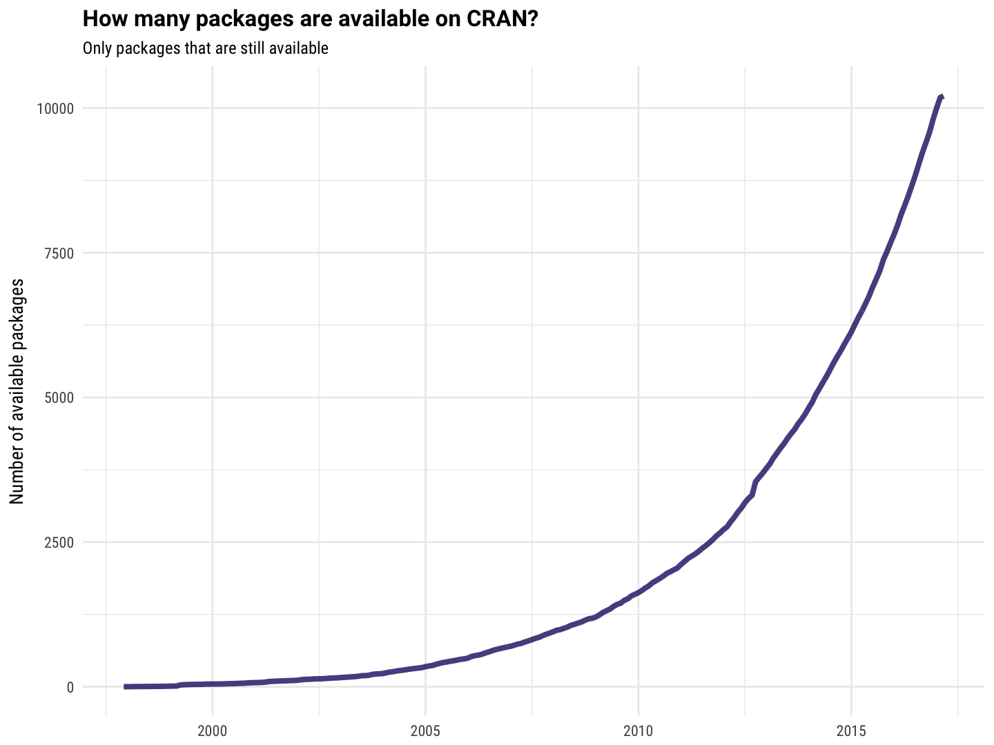
all_pkgs %>%
    filter(!Archived) %>%
    group_by(Date = floor_date(Date, unit = "month")) %>%
    summarise(NewPackages = n()) %>%
    ungroup %>%
    mutate(TotalPackages = cumsum(NewPackages)) %>%
    ggplot(aes(Date, TotalPackages)) +
    geom_line(size = 1.5, alpha = 0.8, color = "midnightblue") +
    labs(x = NULL, y = "Number of available packages",
         title = "How many packages are available on CRAN?",
         subtitle = "Only packages that are still available")

There we go! That is similar to the results we all saw going around when CRAN passed 10,000 packages, which is good.

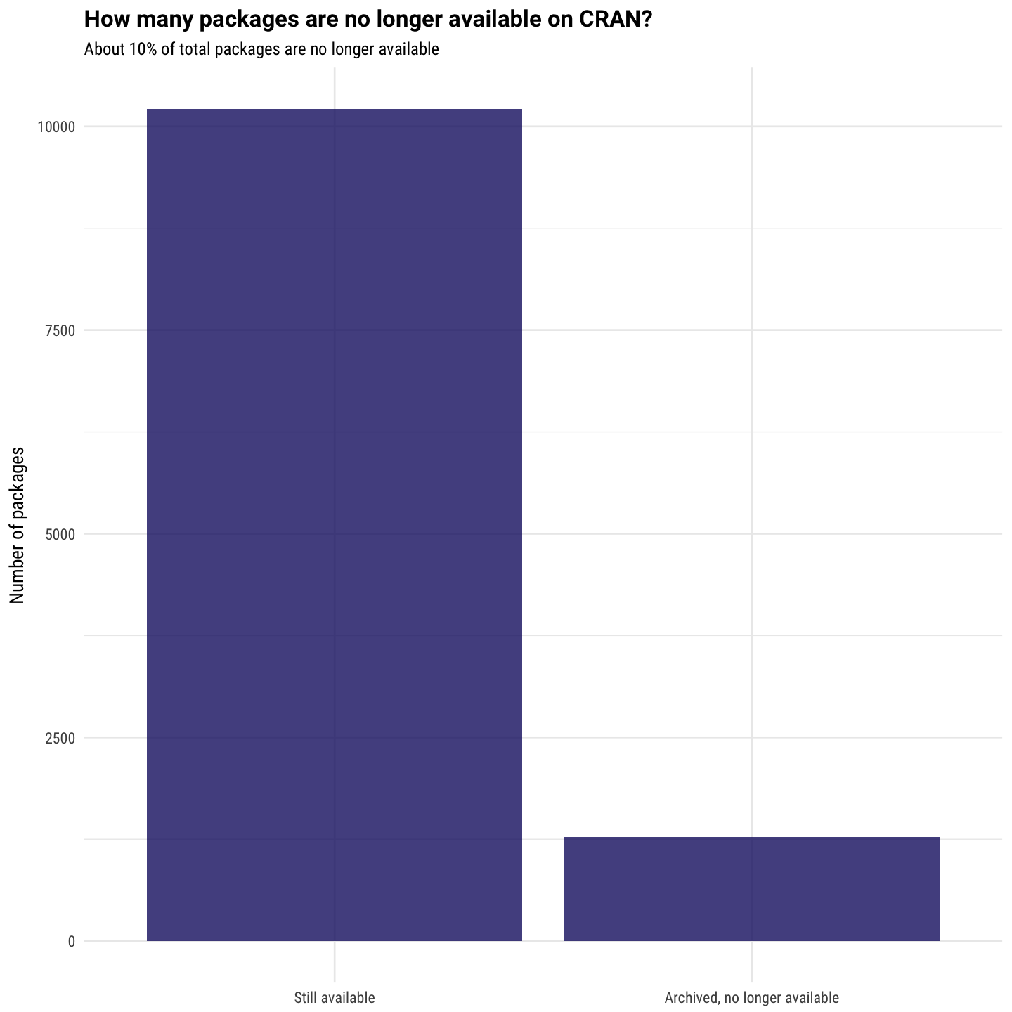
What about the number of archived vs. available packages?

all_pkgs %>%
    ggplot(aes(Archived)) +
    geom_histogram(stat = "count", alpha = 0.8, fill = "midnightblue") +
    scale_x_discrete(labels=c("Still available", "Archived, no longer available")) +
    labs(y = "Number of packages", x = NULL,
         title = "How many packages are no longer available on CRAN?",
         subtitle = "About 10% of total packages are no longer available")

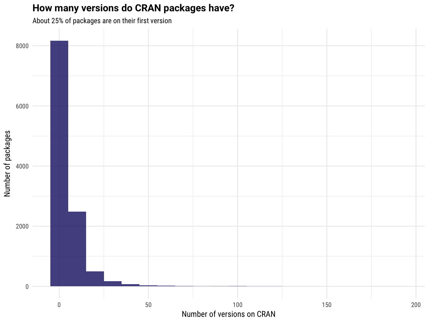
And lastly, let’s look at the distribution of number of releases for each package.

all_pkgs %>%
    ggplot(aes(Versions)) +
    geom_histogram(binwidth = 10, alpha = 0.8, fill = "midnightblue") +
    labs(y = "Number of packages", x = "Number of versions on CRAN",
         title = "How many versions do CRAN packages have?",
         subtitle = "About 25% of packages are on their first version")

The End

It is pretty ironic that I worked on this code and wrote this post because I wanted to do an analysis using different packages than the ones used in the original scripts shared. That is exactly part of the challenge facing all of us as R users now that there is such a diversity of tools out there! I hope that our session at useR this summer provides some clarity and perspective for attendees on these types of issues. The R Markdown file used to make this blog post is available here. Bob Rudis has let me know that there are easier ways to get the data that I used for these plots, and I am very happy to hear about that or other feedback and questions!