Get started with tidymodels and #TidyTuesday Palmer penguins
By Julia Silge in rstats tidymodels
July 28, 2020
Lately I’ve been publishing
screencasts demonstrating how to use the
tidymodels framework, from first steps in modeling to how to evaluate complex models. Today’s screencast is good for folks just getting started with tidymodels, using this week’s
#TidyTuesday dataset on penguins. 🐧
Here is the code I used in the video, for those who prefer reading instead of or in addition to video.
Explore the data
This week’s #TidyTuesday dataset is from palmerpenguins, observations of Antarctic penguins who live on the Palmer Archipelago. You can read more about how this dataset came to be in this post on the RStudio Education blog. Our modeling goal here is to predict the sex of the penguins using a classification model, based on other observations in the dataset.
library(tidyverse)
library(palmerpenguins)

penguins
## # A tibble: 344 x 8
##    species island bill_length_mm bill_depth_mm flipper_length_…
##    <fct>   <fct>           <dbl>         <dbl>            <int>
##  1 Adelie  Torge…           39.1          18.7              181
##  2 Adelie  Torge…           39.5          17.4              186
##  3 Adelie  Torge…           40.3          18                195
##  4 Adelie  Torge…           NA            NA                 NA
##  5 Adelie  Torge…           36.7          19.3              193
##  6 Adelie  Torge…           39.3          20.6              190
##  7 Adelie  Torge…           38.9          17.8              181
##  8 Adelie  Torge…           39.2          19.6              195
##  9 Adelie  Torge…           34.1          18.1              193
## 10 Adelie  Torge…           42            20.2              190
## # … with 334 more rows, and 3 more variables: body_mass_g <int>,
## #   sex <fct>, year <int>
If you try building a classification model for species, you will likely find an almost perfect fit, because these kinds of observations are actually what distinguish different species. Sex, on the other hand, is a little messier.
penguins %>%
  filter(!is.na(sex)) %>%
  ggplot(aes(flipper_length_mm, bill_length_mm, color = sex, size = body_mass_g)) +
  geom_point(alpha = 0.5) +
  facet_wrap(~species)

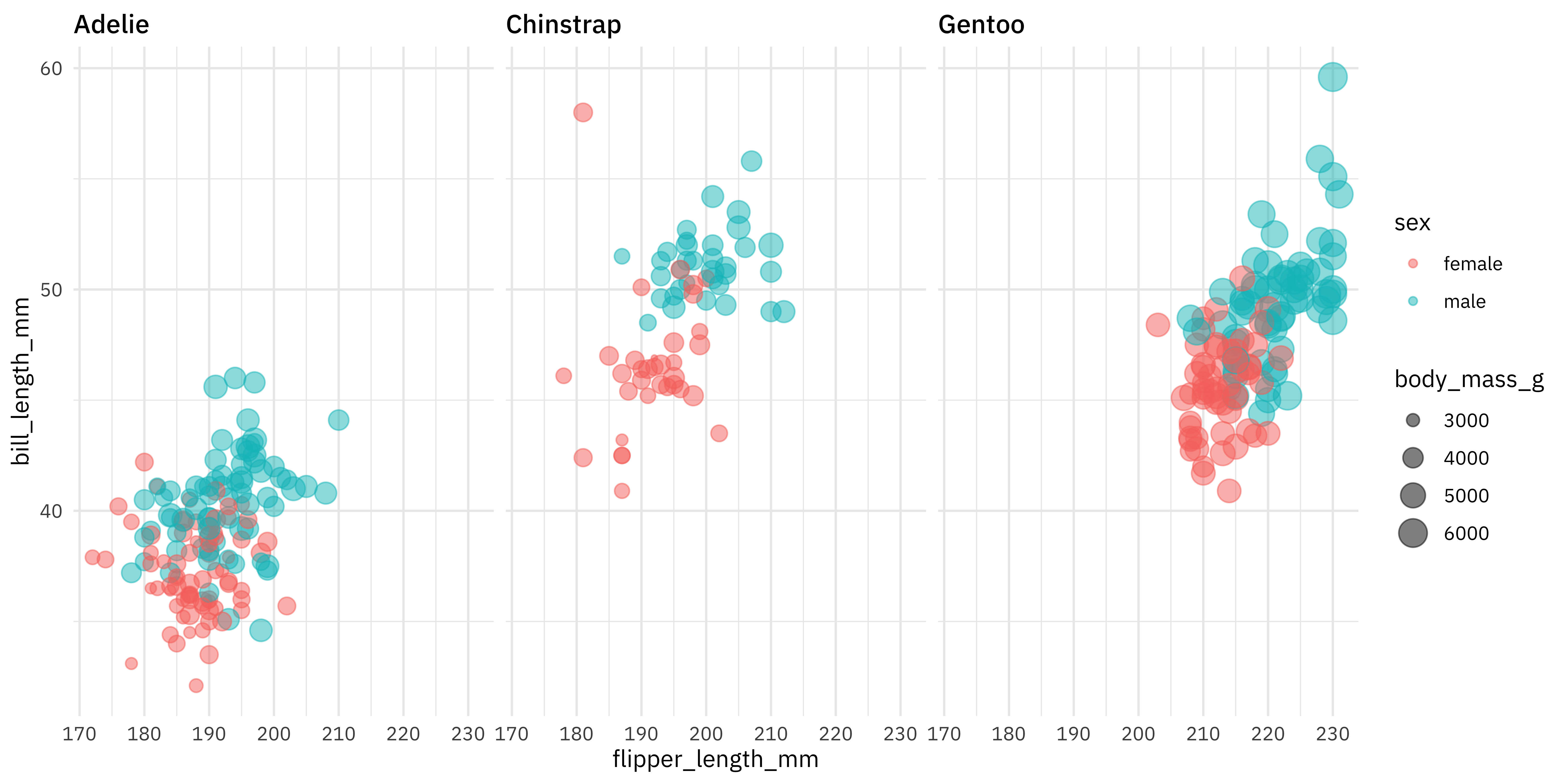
It looks like female penguins are smaller with different bills, but let’s get ready for modeling to find out more! We will not use the island or year information in our model.
penguins_df <- penguins %>%
  filter(!is.na(sex)) %>%
  select(-year, -island)
Build a model
We can start by loading the tidymodels metapackage, and splitting our data into training and testing sets.
library(tidymodels)

set.seed(123)
penguin_split <- initial_split(penguins_df, strata = sex)
penguin_train <- training(penguin_split)
penguin_test <- testing(penguin_split)
Next, let’s create bootstrap resamples of the training data, to evaluate our models.
set.seed(123)
penguin_boot <- bootstraps(penguin_train)
penguin_boot
## # Bootstrap sampling
## # A tibble: 25 x 2
##    splits           id
##    <list>           <chr>
##  1 <split [250/93]> Bootstrap01
##  2 <split [250/92]> Bootstrap02
##  3 <split [250/90]> Bootstrap03
##  4 <split [250/92]> Bootstrap04
##  5 <split [250/86]> Bootstrap05
##  6 <split [250/88]> Bootstrap06
##  7 <split [250/96]> Bootstrap07
##  8 <split [250/89]> Bootstrap08
##  9 <split [250/96]> Bootstrap09
## 10 <split [250/90]> Bootstrap10
## # … with 15 more rows
Let’s compare two different models, a logistic regression model and a random forest model. We start by creating the model specifications.
glm_spec <- logistic_reg() %>%
  set_engine("glm")

glm_spec
## Logistic Regression Model Specification (classification)
##
## Computational engine: glm
rf_spec <- rand_forest() %>%
  set_mode("classification") %>%
  set_engine("ranger")

rf_spec
## Random Forest Model Specification (classification)
##
## Computational engine: ranger
Next let’s start putting together a tidymodels workflow(), a helper object to help manage modeling pipelines with pieces that fit together like Lego blocks. Notice that there is no model yet: Model: None.
penguin_wf <- workflow() %>%
  add_formula(sex ~ .)

penguin_wf
## ══ Workflow ══════════════════════════════════════════════════════════
## Preprocessor: Formula
## Model: None
##
## ── Preprocessor ──────────────────────────────────────────────────────
## sex ~ .
Now we can add a model, and the fit to each of the resamples. First, we can fit the logistic regression model.
glm_rs <- penguin_wf %>%
  add_model(glm_spec) %>%
  fit_resamples(
    resamples = penguin_boot,
    control = control_resamples(save_pred = TRUE)
  )

glm_rs
## # Resampling results
## # Bootstrap sampling
## # A tibble: 25 x 5
##    splits        id        .metrics       .notes       .predictions
##    <list>        <chr>     <list>         <list>       <list>
##  1 <split [250/… Bootstra… <tibble [2 × … <tibble [0 … <tibble [93 × …
##  2 <split [250/… Bootstra… <tibble [2 × … <tibble [0 … <tibble [92 × …
##  3 <split [250/… Bootstra… <tibble [2 × … <tibble [0 … <tibble [90 × …
##  4 <split [250/… Bootstra… <tibble [2 × … <tibble [0 … <tibble [92 × …
##  5 <split [250/… Bootstra… <tibble [2 × … <tibble [0 … <tibble [86 × …
##  6 <split [250/… Bootstra… <tibble [2 × … <tibble [0 … <tibble [88 × …
##  7 <split [250/… Bootstra… <tibble [2 × … <tibble [0 … <tibble [96 × …
##  8 <split [250/… Bootstra… <tibble [2 × … <tibble [0 … <tibble [89 × …
##  9 <split [250/… Bootstra… <tibble [2 × … <tibble [0 … <tibble [96 × …
## 10 <split [250/… Bootstra… <tibble [2 × … <tibble [0 … <tibble [90 × …
## # … with 15 more rows
Second, we can fit the random forest model.
rf_rs <- penguin_wf %>%
  add_model(rf_spec) %>%
  fit_resamples(
    resamples = penguin_boot,
    control = control_resamples(save_pred = TRUE)
  )

rf_rs
## # Resampling results
## # Bootstrap sampling
## # A tibble: 25 x 5
##    splits        id        .metrics       .notes       .predictions
##    <list>        <chr>     <list>         <list>       <list>
##  1 <split [250/… Bootstra… <tibble [2 × … <tibble [0 … <tibble [93 × …
##  2 <split [250/… Bootstra… <tibble [2 × … <tibble [0 … <tibble [92 × …
##  3 <split [250/… Bootstra… <tibble [2 × … <tibble [0 … <tibble [90 × …
##  4 <split [250/… Bootstra… <tibble [2 × … <tibble [0 … <tibble [92 × …
##  5 <split [250/… Bootstra… <tibble [2 × … <tibble [0 … <tibble [86 × …
##  6 <split [250/… Bootstra… <tibble [2 × … <tibble [0 … <tibble [88 × …
##  7 <split [250/… Bootstra… <tibble [2 × … <tibble [0 … <tibble [96 × …
##  8 <split [250/… Bootstra… <tibble [2 × … <tibble [0 … <tibble [89 × …
##  9 <split [250/… Bootstra… <tibble [2 × … <tibble [0 … <tibble [96 × …
## 10 <split [250/… Bootstra… <tibble [2 × … <tibble [0 … <tibble [90 × …
## # … with 15 more rows
We have fit each of our candidate models to our resampled training set!
Evaluate model
Now let’s check out how we did.
collect_metrics(rf_rs)
## # A tibble: 2 x 5
##   .metric  .estimator  mean     n std_err
##   <chr>    <chr>      <dbl> <int>   <dbl>
## 1 accuracy binary     0.893    25 0.00691
## 2 roc_auc  binary     0.958    25 0.00366
Pretty nice! The function collect_metrics() extracts and formats the .metrics column from resampling results like the ones we have here.
collect_metrics(glm_rs)
## # A tibble: 2 x 5
##   .metric  .estimator  mean     n std_err
##   <chr>    <chr>      <dbl> <int>   <dbl>
## 1 accuracy binary     0.897    25 0.00631
## 2 roc_auc  binary     0.964    25 0.00368
So… also great! If I am in a situation where a more complex model like a random forest performs the same as a simpler model like logistic regression, then I will choose the simpler model. Let’s dig deeper into how it is doing. For example, how is it predicting the two classes?
glm_rs %>%
  conf_mat_resampled()
## # A tibble: 4 x 3
##   Prediction Truth   Freq
##   <fct>      <fct>  <dbl>
## 1 female     female 40.6
## 2 female     male    4.48
## 3 male       female  4.92
## 4 male       male   41.4
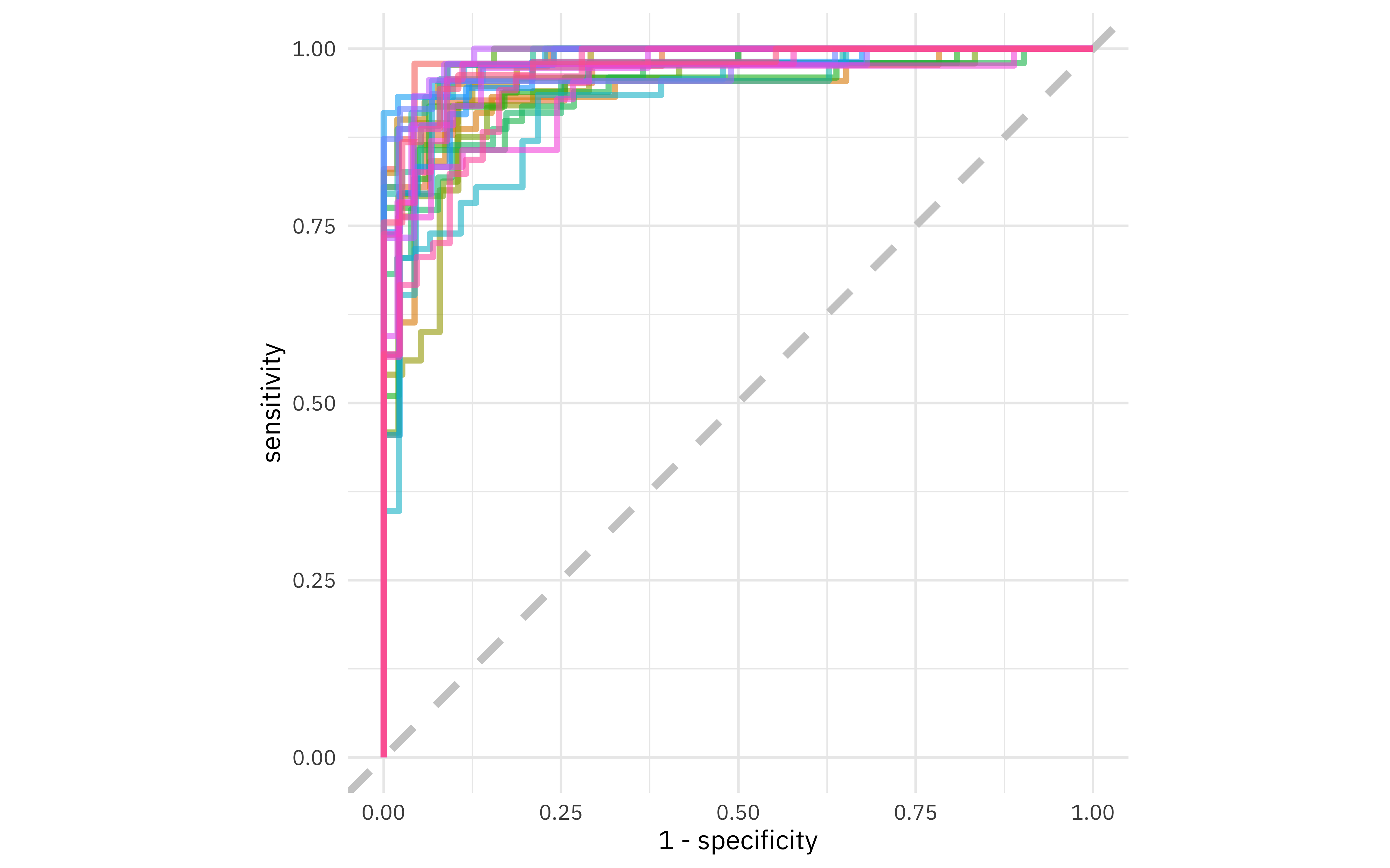
About the same, which is good. We can also make an ROC curve.
glm_rs %>%
  collect_predictions() %>%
  group_by(id) %>%
  roc_curve(sex, .pred_female) %>%
  ggplot(aes(1 - specificity, sensitivity, color = id)) +
  geom_abline(lty = 2, color = "gray80", size = 1.5) +
  geom_path(show.legend = FALSE, alpha = 0.6, size = 1.2) +
  coord_equal()

This ROC curve is more jagged than others you may have seen because the dataset is small.
It is finally time for us to return to the testing set. Notice that we have not used the testing set yet during this whole analysis; the testing set is precious and can only be used to estimate performance on new data. Let’s fit one more time to the training data and evaluate on the testing data using the function last_fit().
penguin_final <- penguin_wf %>%
  add_model(glm_spec) %>%
  last_fit(penguin_split)

penguin_final
## # Resampling results
## # Monte Carlo cross-validation (0.75/0.25) with 1 resamples
## # A tibble: 1 x 6
##   splits     id         .metrics     .notes    .predictions  .workflow
##   <list>     <chr>      <list>       <list>    <list>        <list>
## 1 <split [2… train/tes… <tibble [2 … <tibble … <tibble [83 … <workflo…
The metrics and predictions here are on the testing data.
collect_metrics(penguin_final)
## # A tibble: 2 x 3
##   .metric  .estimator .estimate
##   <chr>    <chr>          <dbl>
## 1 accuracy binary         0.940
## 2 roc_auc  binary         0.991
collect_predictions(penguin_final) %>%
  conf_mat(sex, .pred_class)
##           Truth
## Prediction female male
##     female     39    3
##     male        2   39
The coefficients (which we can get out using tidy()) have been estimated using the training data. If we use exponentiate = TRUE, we have odds ratios.
penguin_final$.workflow[[1]] %>%
  tidy(exponentiate = TRUE)
## # A tibble: 7 x 5
##   term              estimate std.error statistic       p.value
##   <chr>                <dbl>     <dbl>     <dbl>         <dbl>
## 1 (Intercept)       3.12e-35  13.5         -5.90 0.00000000369
## 2 speciesChinstrap  1.34e- 3   1.70        -3.89 0.000101
## 3 speciesGentoo     1.08e- 4   2.89        -3.16 0.00159
## 4 bill_length_mm    1.78e+ 0   0.137        4.20 0.0000268
## 5 bill_depth_mm     3.89e+ 0   0.373        3.64 0.000273
## 6 flipper_length_mm 1.07e+ 0   0.0538       1.31 0.189
## 7 body_mass_g       1.01e+ 0   0.00108      4.70 0.00000260
- The largest odds ratio is for bill depth, with the second largest for bill length. An increase of 1 mm in bill depth corresponds to almost 4x higher odds of being male. The characteristics of a penguin’s bill must be associated with their sex.
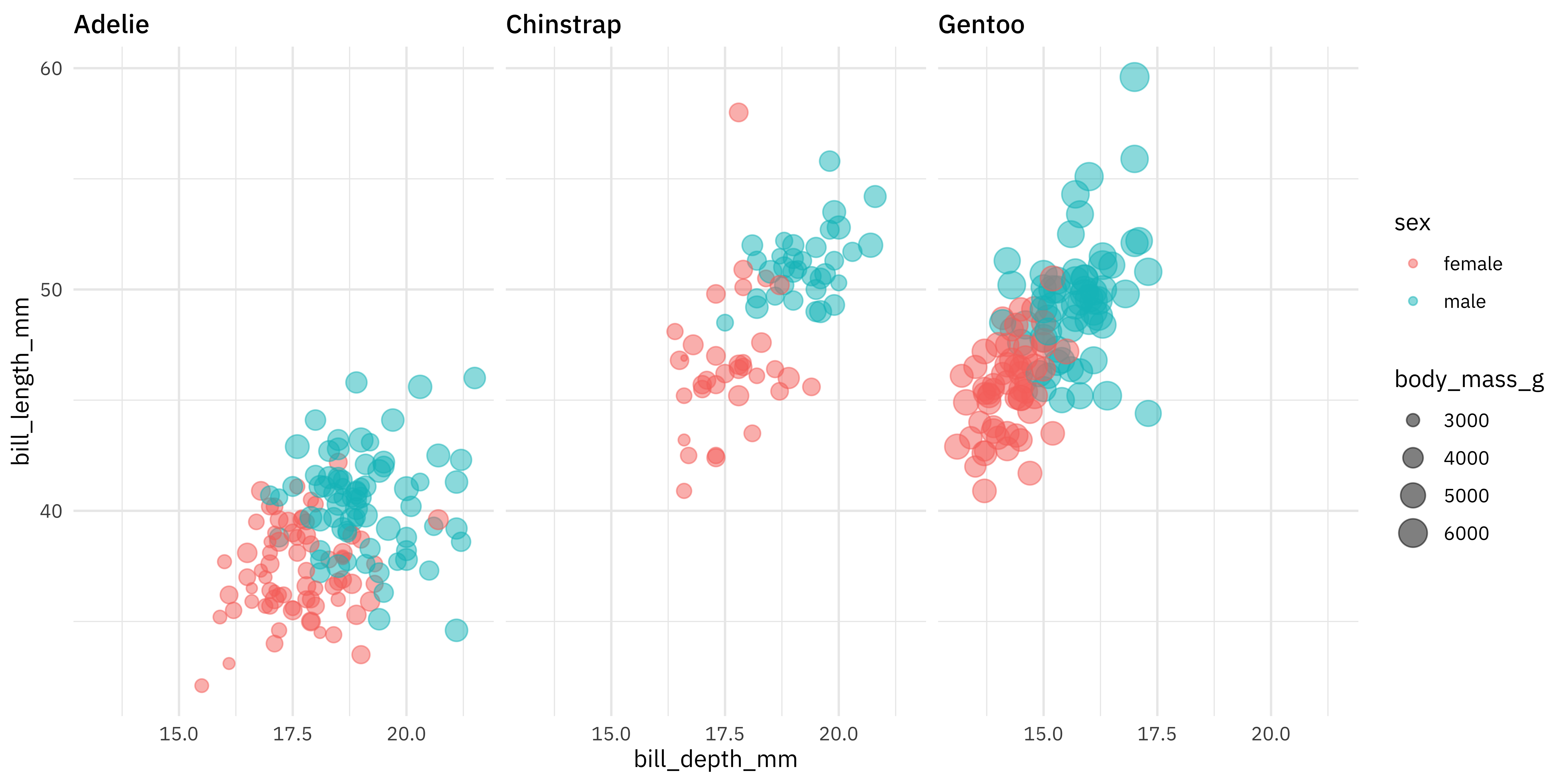
- We don’t have strong evidence that flipper length is different between male and female penguins, controlling for the other measures; maybe we should explore that by changing that first plot!
penguins %>%
  filter(!is.na(sex)) %>%
  ggplot(aes(bill_depth_mm, bill_length_mm, color = sex, size = body_mass_g)) +
  geom_point(alpha = 0.5) +
  facet_wrap(~species)

Yes, the male and female penguins are much more separated now.
- Posted on:
- July 28, 2020
- Length:
- 8 minute read, 1673 words
- Categories:
- rstats tidymodels
- Tags:
- rstats tidymodels