The Life-Changing Magic of Tidying Text
By Julia Silge
April 29, 2016
When I went to the rOpenSci unconference about a month ago, I started work with Dave Robinson on a package for text mining using tidy data principles. What is this tidy data you keep hearing so much about? As described by Hadley Wickham, tidy data has a specific structure:
- each variable is a column
- each observation is a row
- each type of observational unit is a table
This means we end up with a data set that is in a long, skinny format instead of a wide format. Tidy data sets are easier to work with, and this is no less true when one starts to work with text. Most of the tooling and infrastructure needed for text mining with tidy data frames already exists in packages like dplyr, broom, tidyr, and ggplot2. Our goal in writing the tidytext package is to provide functions and supporting data sets to allow conversion of text to and from tidy formats, and to switch seamlessly between tidy tools and existing text mining packages. We got a great start on our work when we were at the unconference and recently finished getting the first release ready; this week, tidytext was released on CRAN!
Jane Austen’s Novels Can Be So Tidy
One of the important functions we knew we needed was something to unnest text by some chosen token. In my
previous blog
posts, I did this with a for loop first and then with a function that involved several dplyr bits. In the tidytext package, there is a function unnest_tokens which has this functionality; it restructures text into a one-token-per-row format. This function is a way to convert a dataframe with a text column to be one-token-per-row. Let’s look at an example using Jane Austen’s novels.
(What?! Surely you’re not tired of them yet?)
The janeaustenr package has a function austen_books that returns a tidy dataframe of all of the novels. Let’s use that, annotate a linenumber quantity to keep track of lines in the original format, use a regex to find where all the chapters are, and then unnest_tokens.
library(janeaustenr)
library(tidytext)
library(dplyr)
library(stringr)

original_books <- austen_books() %>%
        group_by(book) %>%
        mutate(linenumber = row_number(),
               chapter = cumsum(str_detect(text, regex("^chapter [\\divxlc]",
                                                 ignore_case = TRUE)))) %>%
        ungroup()

original_books
## Source: local data frame [70,942 x 4]
##
##                     text                book linenumber chapter
##                    (chr)              (fctr)      (int)   (int)
## 1  SENSE AND SENSIBILITY Sense & Sensibility          1       0
## 2                        Sense & Sensibility          2       0
## 3         by Jane Austen Sense & Sensibility          3       0
## 4                        Sense & Sensibility          4       0
## 5                 (1811) Sense & Sensibility          5       0
## 6                        Sense & Sensibility          6       0
## 7                        Sense & Sensibility          7       0
## 8                        Sense & Sensibility          8       0
## 9                        Sense & Sensibility          9       0
## 10             CHAPTER 1 Sense & Sensibility         10       1
## ..                   ...                 ...        ...     ...
tidy_books <- original_books %>%
        unnest_tokens(word, text)

tidy_books
## Source: local data frame [724,971 x 4]
##
##                   book linenumber chapter        word
##                 (fctr)      (int)   (int)       (chr)
## 1  Sense & Sensibility          1       0       sense
## 2  Sense & Sensibility          1       0         and
## 3  Sense & Sensibility          1       0 sensibility
## 4  Sense & Sensibility          3       0          by
## 5  Sense & Sensibility          3       0        jane
## 6  Sense & Sensibility          3       0      austen
## 7  Sense & Sensibility          5       0        1811
## 8  Sense & Sensibility         10       1     chapter
## 9  Sense & Sensibility         10       1           1
## 10 Sense & Sensibility         13       1         the
## ..                 ...        ...     ...         ...
This function uses the tokenizers package to separate each line into words. The default tokenizing is for words, but other options include characters, sentences, lines, paragraphs, or separation around a regex pattern.
Now that the data is in one-word-per-row format, the TIDY DATA MAGIC can happen and we can manipulate it with tidy tools like dplyr. For example, we can remove stop words (kept in the tidytext dataset stop_words) with an anti_join.
data("stop_words")
tidy_books <- tidy_books %>%
        anti_join(stop_words)
Then we can use count to find the most common words in all of Jane Austen’s novels as a whole.
tidy_books %>%
        count(word, sort = TRUE)
## Source: local data frame [13,896 x 2]
##
##      word     n
##     (chr) (int)
## 1    miss  1854
## 2    time  1337
## 3   fanny   862
## 4    dear   822
## 5    lady   817
## 6     sir   806
## 7     day   797
## 8    emma   787
## 9  sister   727
## 10  house   699
## ..    ...   ...
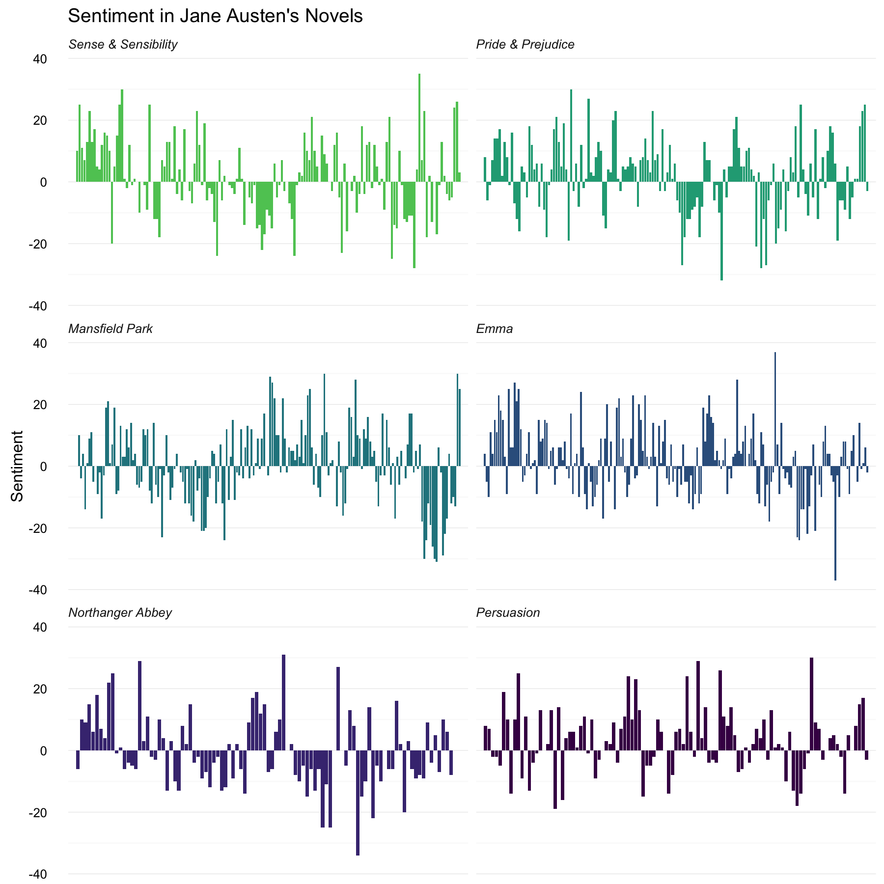
Sentiment analysis can be done as an inner join. Three sentiment lexicons are in the tidytext package in the sentiment dataset. Let’s examine how sentiment changes changes during each novel. Let’s find a sentiment score for each word using the Bing lexicon, then count the number of positive and negative words in defined sections of each novel.
library(tidyr)
bing <- sentiments %>%
        filter(lexicon == "bing") %>%
        select(-score)

bing
## Source: local data frame [6,788 x 3]
##
##           word sentiment lexicon
##          (chr)     (chr)   (chr)
## 1      2-faced  negative    bing
## 2      2-faces  negative    bing
## 3           a+  positive    bing
## 4     abnormal  negative    bing
## 5      abolish  negative    bing
## 6   abominable  negative    bing
## 7   abominably  negative    bing
## 8    abominate  negative    bing
## 9  abomination  negative    bing
## 10       abort  negative    bing
## ..         ...       ...     ...
janeaustensentiment <- tidy_books %>%
        inner_join(bing) %>%
        count(book, index = linenumber %/% 80, sentiment) %>%
        spread(sentiment, n, fill = 0) %>%
        mutate(sentiment = positive - negative)

janeaustensentiment
## Source: local data frame [891 x 5]
## Groups: book, index [891]
##
##                   book index negative positive sentiment
##                 (fctr) (dbl)    (dbl)    (dbl)     (dbl)
## 1  Sense & Sensibility     0       16       26        10
## 2  Sense & Sensibility     1       19       44        25
## 3  Sense & Sensibility     2       12       23        11
## 4  Sense & Sensibility     3       15       22         7
## 5  Sense & Sensibility     4       16       29        13
## 6  Sense & Sensibility     5       16       39        23
## 7  Sense & Sensibility     6       24       37        13
## 8  Sense & Sensibility     7       22       39        17
## 9  Sense & Sensibility     8       30       35         5
## 10 Sense & Sensibility     9       14       18         4
## ..                 ...   ...      ...      ...       ...
Now we can plot these sentiment scores across the plot trajectory of each novel.
library(ggplot2)
library(viridis)
ggplot(janeaustensentiment, aes(index, sentiment, fill = book)) +
        geom_bar(stat = "identity", show.legend = FALSE) +
        facet_wrap(~book, ncol = 2, scales = "free_x") +
        theme_minimal(base_size = 13) +
        labs(title = "Sentiment in Jane Austen's Novels",
             y = "Sentiment") +
        scale_fill_viridis(end = 0.75, discrete=TRUE, direction = -1) +
        scale_x_discrete(expand=c(0.02,0)) +
        theme(strip.text=element_text(hjust=0)) +
        theme(strip.text = element_text(face = "italic")) +
        theme(axis.title.x=element_blank()) +
        theme(axis.ticks.x=element_blank()) +
        theme(axis.text.x=element_blank())

This is similar to some of the plots I have made in previous posts, but the effort and time required to make it is drastically less. More importantly, the thinking required to make it comes much more easily because it all falls so naturally out of joins and other dplyr verbs.
Looking at Units Beyond Words
Lots of useful work can be done by tokenizing at the word level, but sometimes it is useful or necessary to look at different units of text. For example, some sentiment analysis algorithms look beyond only unigrams (i.e. single words) to try to understand the sentiment of a sentence as a whole. These algorithms try to understand that
I am not having a good day.
is a negative sentence, not a positive one, because of negation. The Stanford CoreNLP tools and the sentimentr R package (currently available on Github but not CRAN) are examples of such sentiment analysis algorithms. For these, we may want to tokenize text into sentences.
austen_sentences <- austen_books() %>%
        group_by(book) %>%
        unnest_tokens(sentence, text, token = "sentences") %>%
        ungroup()
Let’s look at just one.
austen_sentences$sentence[39]
## [1] "it would be enough to make them completely easy."
The sentence tokenizing does seem to have a bit of trouble with UTF-8 encoded text, especially with sections of dialogue; it does much better with punctuation in ASCII.
Near the beginning of this vignette, we used a regex to find where all the chapters were in Austen’s novels. We can use tidy text analysis to ask questions such as what are the most negative chapters in each of Jane Austen’s novels? First, let’s get the list of negative words from the Bing lexicon. Second, let’s make a dataframe of how many words are in each chapter so we can normalize for the length of chapters. Then, let’s find the number of negative words in each chapter and divide by the total words in each chapter. Which chapter has the highest proportion of negative words?
bingnegative <- sentiments %>%
        filter(lexicon == "bing", sentiment == "negative")

wordcounts <- tidy_books %>%
        group_by(book, chapter) %>%
        summarize(words = n())

tidy_books %>%
        semi_join(bingnegative) %>%
        group_by(book, chapter) %>%
        summarize(negativewords = n()) %>%
        left_join(wordcounts, by = c("book", "chapter")) %>%
        mutate(ratio = negativewords/words) %>%
        filter(chapter != 0) %>%
        top_n(1)
## Source: local data frame [6 x 5]
## Groups: book [6]
##
##                  book chapter negativewords words     ratio
##                (fctr)   (int)         (int) (int)     (dbl)
## 1 Sense & Sensibility      29           172  1135 0.1515419
## 2   Pride & Prejudice      34           108   646 0.1671827
## 3      Mansfield Park      45           132   884 0.1493213
## 4                Emma      15           147  1012 0.1452569
## 5    Northanger Abbey      27            55   337 0.1632047
## 6          Persuasion      21           215  1948 0.1103696
These are the chapters with the most negative words in each book, normalized for number of words in the chapter. What is happening in these chapters? In Chapter 29 of Sense and Sensibility Marianne finds out what an awful jerk Willoughby is by letter, and in Chapter 34 of Pride and Prejudice Mr. Darcy proposes for the first time (so badly!). Chapter 45 of Mansfield Park is almost the end, when Tom is sick with consumption and Mary is revealed as all greedy and a gold-digger, Chapter 15 of Emma is when horrifying Mr. Elton proposes, and Chapter 27 of Northanger Abbey is a short chapter where Catherine gets a terrible letter from her inconstant friend Isabella. Chapter 21 of Persuasion is when Anne’s friend tells her all about Mr. Elliott’s immoral past.
Interestingly, many of those chapters are very close to the ends of the novels; things tend to get really bad for Jane Austen’s characters before their happy endings, it seems. Also, these chapters largely involve terrible revelations about characters through letters or conversations about past events, rather than some action happening directly in the plot. All that, just with dplyr verbs, because the data is tidy.
Networks of Words
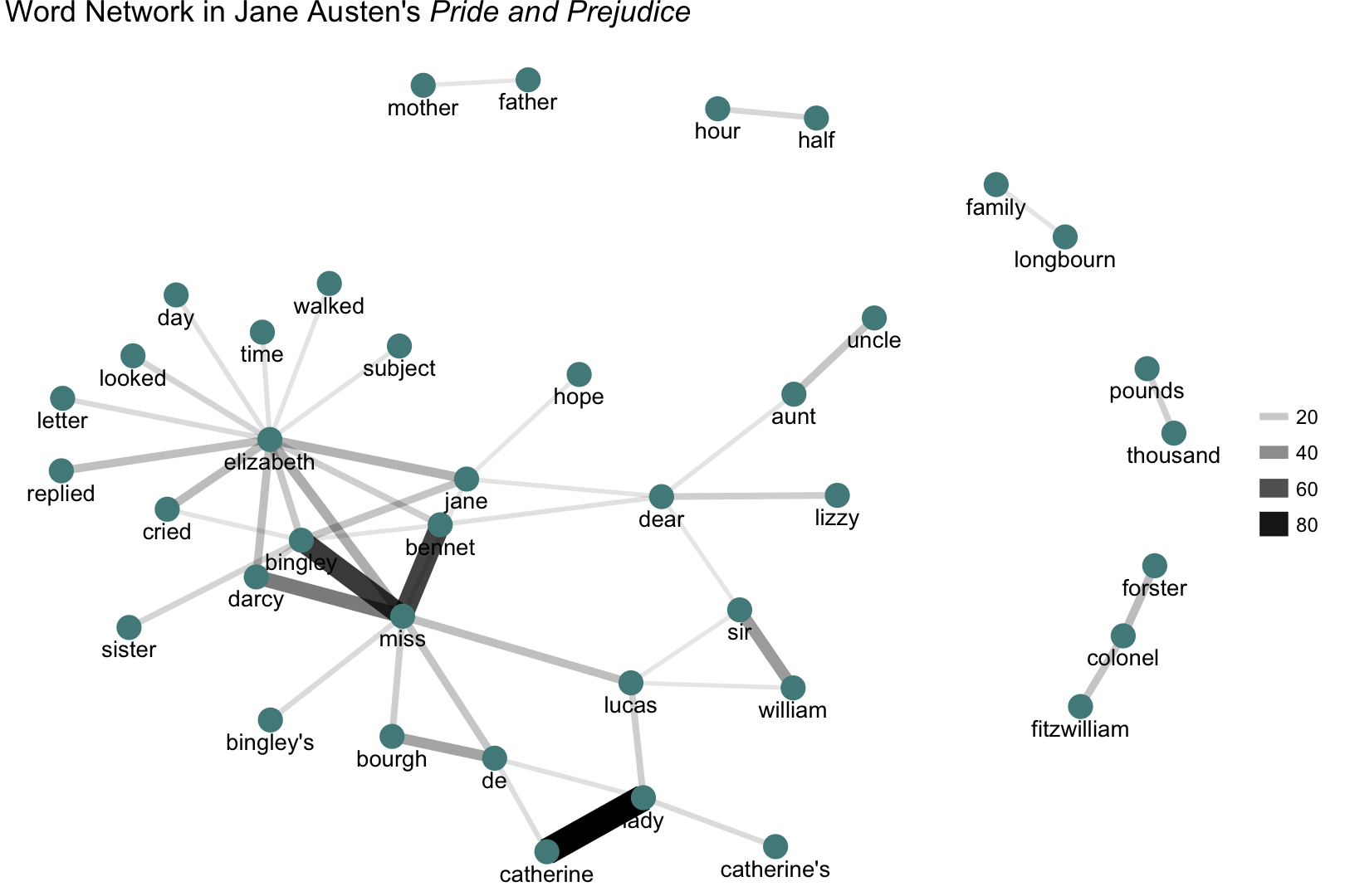
Another function in tidytext is pair_count, which counts pairs of items that occur together within a group. Let’s count the words that occur together in the lines of Pride and Prejudice.
pride_prejudice_words <- tidy_books %>%
        filter(book == "Pride & Prejudice")
word_cooccurences <- pride_prejudice_words %>%
        pair_count(linenumber, word, sort = TRUE)
word_cooccurences
## Source: local data frame [50,550 x 3]
##
##       value1  value2     n
##        (chr)   (chr) (dbl)
## 1  catherine    lady    87
## 2    bingley    miss    68
## 3     bennet    miss    65
## 4      darcy    miss    46
## 5    william     sir    35
## 6     bourgh      de    32
## 7  elizabeth    miss    29
## 8  elizabeth    jane    27
## 9  elizabeth   cried    24
## 10   forster colonel    24
## ..       ...     ...   ...
This can be useful, for example, to plot a network of co-occuring words with the igraph and ggraph packages.
library(igraph)
library(ggraph)

set.seed(1813)
word_cooccurences %>%
        filter(n >= 10) %>%
        graph_from_data_frame() %>%
        ggraph(layout = "fr") +
        geom_edge_link(aes(edge_alpha = n, edge_width = n)) +
        geom_node_point(color = "darkslategray4", size = 5) +
        geom_node_text(aes(label = name), vjust = 1.8) +
        ggtitle(expression(paste("Word Network in Jane Austen's ",
                                 italic("Pride and Prejudice")))) +
        theme_void()

Ten/five/whatever thousand pounds a year!
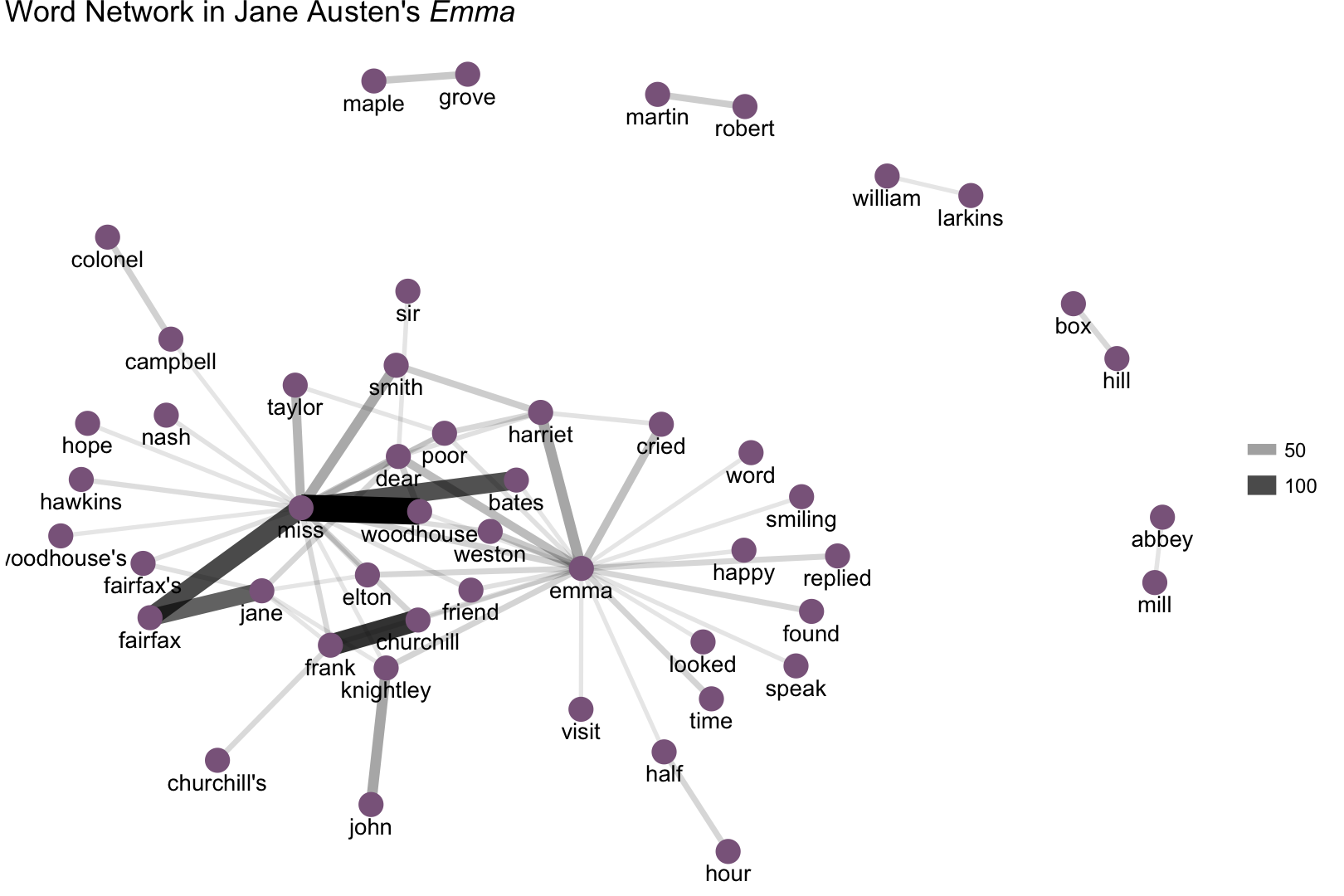
Let’s do another one!
pride_prejudice_words <- tidy_books %>%
        filter(book == "Emma")
word_cooccurences <- pride_prejudice_words %>%
        pair_count(linenumber, word, sort = TRUE)
set.seed(2016)
word_cooccurences %>%
        filter(n >= 10) %>%
        graph_from_data_frame() %>%
        ggraph(layout = "fr") +
        geom_edge_link(aes(edge_alpha = n, edge_width = n)) +
        geom_node_point(color = "plum4", size = 5) +
        geom_node_text(aes(label = name), vjust = 1.8) +
        ggtitle(expression(paste("Word Network in Jane Austen's ",
                                 italic("Emma")))) +
        theme_void()

Lots of proper nouns are showing up in these network plots (Box Hill, Frank Churchill, Lady Catherine de Bourgh, etc.), and it is easy to pick out the main characters (Elizabeth, Emma). This type of network analysis is mainly showing us the important people and places in a text, and how they are related.
Word Frequencies
A common task in text mining is to look at word frequencies and to compare frequencies across different texts. We can do this using tidy data principles pretty smoothly. We already have Jane Austen’s works; let’s get two more sets of texts to compare to. Dave has just put together a new package to search and download books from Project Gutenberg through R; we’re going to use that because this is a better way to follow Project Gutenberg’s rules for robot access. And it is SO nice to use! First, let’s look at some science fiction and fantasy novels by H.G. Wells, who lived in the late 19th and early 20th centuries. Let’s get The Time Machine, The War of the Worlds, The Invisible Man, and The Island of Doctor Moreau.
library(gutenbergr)
hgwells <- gutenberg_download(c(35, 36, 5230, 159))
tidy_hgwells <- hgwells %>%
        unnest_tokens(word, text) %>%
        anti_join(stop_words)
Just for kicks, what are the most common words in these novels of H.G. Wells?
tidy_hgwells %>%
        count(word, sort = TRUE)
## Source: local data frame [11,769 x 2]
##
##      word     n
##     (chr) (int)
## 1    time   454
## 2  people   302
## 3    door   260
## 4   heard   249
## 5   black   232
## 6   stood   229
## 7   white   222
## 8    hand   218
## 9    kemp   213
## 10   eyes   210
## ..    ...   ...
Now let’s get some well-known works of the Brontë sisters, whose lives overlapped with Jane Austen’s somewhat but who wrote in a bit of a different style. Let’s get Jane Eyre, Wuthering Heights, The Tenant of Wildfell Hall, Villette, and Agnes Grey.
bronte <- gutenberg_download(c(1260, 768, 969, 9182, 766))
tidy_bronte <- bronte %>%
        unnest_tokens(word, text) %>%
        anti_join(stop_words)
What are the most common words in these novels of the Brontë sisters?
tidy_bronte %>%
        count(word, sort = TRUE)
## Source: local data frame [25,714 x 2]
##
##      word     n
##     (chr) (int)
## 1    time  1586
## 2    miss  1388
## 3    hand  1239
## 4     day  1136
## 5    eyes  1023
## 6   night  1011
## 7   house   960
## 8    head   957
## 9  looked   949
## 10   aunt   896
## ..    ...   ...
Well, Jane Austen is not going around talking about people’s HEARTS this much; I can tell you that right now. Those Brontë sisters, SO DRAMATIC. Interesting that “time” and “door” are in the top 10 for both H.G. Wells and the Brontë sisters. “Door”?!
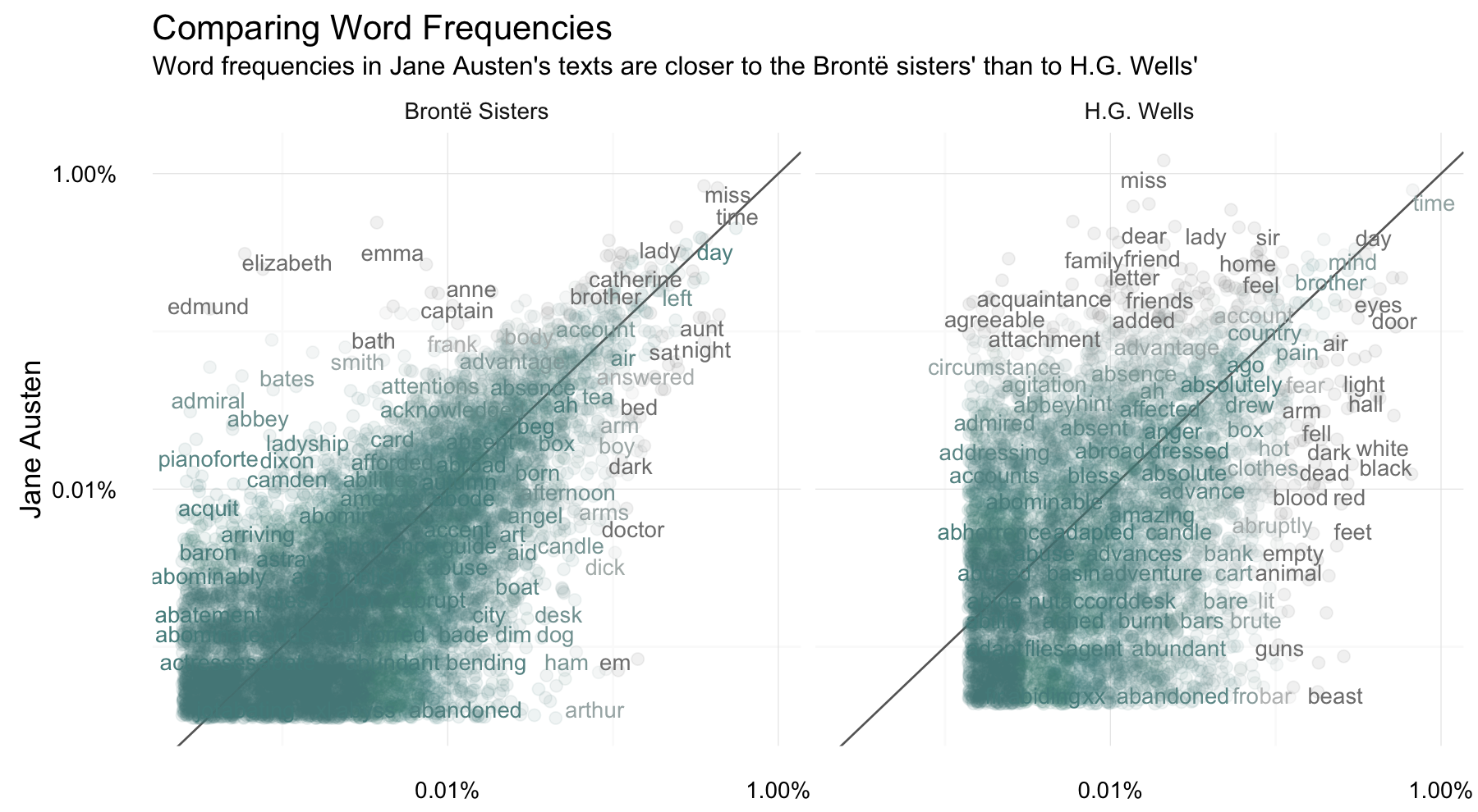
Anyway, let’s calculate the frequency for each word for the works of Jane Austen, the Brontë sisters, and H.G. Wells.
tidy_both <- bind_rows(
        mutate(tidy_bronte, author = "Brontë Sisters"),
        mutate(tidy_hgwells, author = "H.G. Wells"))
frequency <- tidy_both %>%
        mutate(word = str_extract(word, "[a-z]+")) %>%
        count(author, word) %>%
        rename(other = n) %>%
        inner_join(count(tidy_books, word)) %>%
        rename(Austen = n) %>%
        mutate(other = other / sum(other),
               Austen = Austen / sum(Austen)) %>%
        ungroup()
I’m using str_extract here because the UTF-8 encoded texts from Project Gutenberg have some examples of words with underscores around them to indicate emphasis (you know, like italics). The tokenizer treated these as words but I don’t want to count “_any_” separately from “any”. Now let’s plot.
library(scales)
ggplot(frequency, aes(x = other, y = Austen, color = abs(Austen - other))) +
        geom_abline(color = "gray40") +
        geom_jitter(alpha = 0.1, size = 2.5, width = 0.4, height = 0.4) +
        geom_text(aes(label = word), check_overlap = TRUE, vjust = 1.5) +
        scale_x_log10(labels = percent_format()) +
        scale_y_log10(labels = percent_format()) +
        scale_color_gradient(limits = c(0, 0.001), low = "darkslategray4", high = "gray75") +
        facet_wrap(~author, ncol = 2) +
        theme_minimal(base_size = 14) +
        theme(legend.position="none") +
        labs(title = "Comparing Word Frequencies",
             subtitle = "Word frequencies in Jane Austen's texts are closer to the Brontë sisters' than to H.G. Wells'",
             y = "Jane Austen", x = NULL)

Words that are close to the line in these plots have similar frequencies in both sets of texts, for example, in both Austen and Brontë texts (“miss”, “time”, “lady”, “day” at the upper frequency end) or in both Austen and Wells texts (“time”, “day”, “mind”, “brother” at the high frequency end). Words that are far from the line are words that are found more in one set of texts than another. For example, in the Austen-Brontë plot, words like “elizabeth”, “emma”, “captain”, and “bath” (all proper nouns) are found in Austen’s texts but not much in the Brontë texts, while words like “arthur”, “dark”, “dog”, and “doctor” are found in the Brontë texts but not the Austen texts. In comparing H.G. Wells with Jane Austen, Wells uses words like “beast”, “guns”, “brute”, and “animal” that Austen does not, while Austen uses words like “family”, “friend”, “letter”, and “agreeable” that Wells does not.
Overall, notice that the words in the Austen-Brontë plot are closer to the zero-slope line than in the Austen-Wells plot and also extend to lower frequencies; Austen and the Brontë sisters use more similar words than Austen and H.G. Wells. Also, you might notice the percent frequencies for individual words are different in one plot when compared to another because of the inner join; not all the words are found in all three sets of texts so the percent frequency is a different quantity.
Let’s quantify how similar and different these sets of word frequencies are using a correlation test. How correlated are the word frequencies between Austen and the Brontë sisters, and between Austen and Wells?
cor.test(data = frequency[frequency$author == "Brontë Sisters",], ~ other + Austen)
##
## 	Pearson's product-moment correlation
##
## data:  other and Austen
## t = 122.45, df = 10611, p-value < 2.2e-16
## alternative hypothesis: true correlation is not equal to 0
## 95 percent confidence interval:
##  0.7572399 0.7730119
## sample estimates:
##       cor
## 0.7652408
cor.test(data = frequency[frequency$author == "H.G. Wells",], ~ other + Austen)
##
## 	Pearson's product-moment correlation
##
## data:  other and Austen
## t = 36.043, df = 5958, p-value < 2.2e-16
## alternative hypothesis: true correlation is not equal to 0
## 95 percent confidence interval:
##  0.4020291 0.4437216
## sample estimates:
##       cor
## 0.4230993
The relationship between the word frequencies is different between these sets of texts, as it appears in the plots.
The End
There is another whole set of functions in tidytext for converting to and from document-term matrices. Many existing text mining data sets are in document-term matrices, or you might want such a matrix for a specific machine learning application. The tidytext package has tidy functions for objects from the tm and quanteda packages so you can convert back and forth. (For more on the tidy verb, see the
broom package). This allows, for example, a workflow with easy reading, filtering, and processing to be done using dplyr and other tidy tools, after which the data can be converted into a document-term matrix for machine learning applications. For examples of working with objects from other text mining packages using tidy data principles, see the tidytext vignette on converting to and from document-term matrices.
Many thanks to rOpenSci for hosting the unconference where we started work on the tidytext package, and to Gabriela de Queiroz, who contributed to the package while we were at the unconference. I am super happy to have collaborated with Dave; it has been a delightful experience. The R Markdown file used to make this blog post is available here. I am very happy to hear feedback or questions!