Joy to the World, and also Anticipation, Disgust, Surprise...
Natural Language Processing and Sentiment Analysis of My Twitter Archive
By Julia Silge in rstats
December 22, 2015
In my previous blog post, I analyzed my Twitter archive and explored some aspects of my tweeting behavior. When do I tweet, how much do retweet people, do I use hashtags? These are examples of one kind of question, but what about the actual verbal content of my tweets, the text itself? What kinds of questions can we ask and answer about the text in some programmatic way? This is what is called natural language processing, and I’ll give a first shot at it here. First, let’s load some libraries I’ll use in this analysis and open up my Twitter archive.
library(tm)
library(stringr)
library(wordcloud)

tweets <- read.csv("./tweets.csv", stringsAsFactors = FALSE)
Cloudy With a Chance of Lots of Words
Perhaps the simplest question we might want to ask is about the frequency of words used in text. What words do I use a lot in my tweets? Let’s find out, and make a common visualization of term frequency called a word cloud.
First, let’s remove the Twitter handles (i.e., @juliasilge or similar) from the tweet texts so we can just have the real English words.
nohandles <- str_replace_all(tweets$text, "@\\w+", "")
Now, let’s go through and clean up the remaining text. We will turn this into a “corpus”, a collection of documents containing natural language text that the tm text mining package knows how to deal with. After that, we’ll go through and apply specific mappings to the documents (i.e., tweet texts). These can actually be done all in one call to tm_map but I have them separated here to show clearly what is going on.
wordCorpus <- Corpus(VectorSource(nohandles))
wordCorpus <- tm_map(wordCorpus, removePunctuation)
wordCorpus <- tm_map(wordCorpus, content_transformer(tolower))
wordCorpus <- tm_map(wordCorpus, removeWords, stopwords("english"))
wordCorpus <- tm_map(wordCorpus, removeWords, c("amp", "2yo", "3yo", "4yo"))
wordCorpus <- tm_map(wordCorpus, stripWhitespace)
The mappings do pretty much what they sound like they do. First, we remove all punctuation, then we change everything to all lower case. The next line removes English stop words; these are very common words that aren’t super meaningful. If we didn’t remove stop words, then most people’s text will look pretty much the same and my word cloud would just be an enormous the with various prepositions and conjunctions and such around it. In the next line, let’s remove some “words” that were leftover from how special characters were treated in the Twitter archive. The last line strips whitespace from before and after each word so that now the corpus holds nice, neat, cleaned-up words.
A common transformation or mapping to do when examining term frequency is called stemming; this means to take words like cleaning and cleaned and cleaner and remove the endings of the words to keep just clean for all of these examples. Then we can count all of them together instead of separately, which sounds like it would be an excellent thing to do. The stemming algorithm in tm did not work very well for my purposes for my tweet texts, however. It turned some common words in my tweet texts into misspellings; it changed baby to babi, morning to morn, little to littl, etc.
# did not do this stemming
wordCorpus <- tm_map(wordCorpus, stemDocument)
This might actually be a sensible, great thing to do if my ultimate goal was to algorithmically compare my corpus to another corpus. It wouldn’t much matter if the words being counted were correctly spelled English words, and it would make more difference pay attention to stemming. However, I want to make a word cloud for us all to look at, so I don’t want to have anything nonsensical or incorrectly spelled; I will leave out stemming. It did not make a big difference in my results here when I did and did not include stemming. That’s actually pretty interesting; it must be related to the tense and inflection that I use in tweets.
So now let’s make the word cloud. The wordcloud function takes either a corpus like we have here, or a vector of words and their frequencies, or even a bunch of text, and then plots a word cloud. We can tinker with the scale of the sizes of the words to be plotted, the colors used, and how many words to plot. For what it’s worth, I could not get wordcloud to play nicely with svglite, so I am using the default PNG format from knitr here.
pal <- brewer.pal(9,"YlGnBu")
pal <- pal[-(1:4)]
set.seed(123)
wordcloud(words = wordCorpus, scale=c(5,0.1), max.words=100, random.order=FALSE,
          rot.per=0.35, use.r.layout=FALSE, colors=pal)
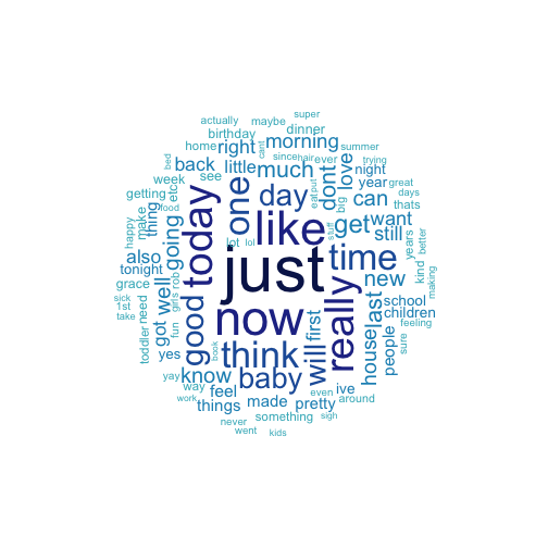
I just… Like, really?
You can see that there are a few examples where stemming would have made sense, thing and things, for example. Also, we can definitely see here that I have been a social, personal user of Twitter since I joined in 2008. These words all look conversational, personal, and informal. We would see a very different word cloud for someone who has used Twitter for professional purposes over her whole Twitter career. Another way to quantify the information shown in the word cloud is called a term-document matrix; this is a matrix of numbers (0 and 1) that keeps track of which documents in a corpus use which terms. Let’s see this for the corpus of my tweets.
tdm <- TermDocumentMatrix(wordCorpus)
tdm
## <<TermDocumentMatrix (terms: 14712, documents: 10202)>>
## Non-/sparse entries: 82638/150009186
## Sparsity           : 100%
## Maximal term length: 78
## Weighting          : term frequency (tf)
So this term-document matrix contains information on 14712 terms (i.e, words) and 10202 documents (i.e., tweets). We could also make a document-term matrix, which has the rows and columns the other way around. Let’s look at part of this matrix.
inspect(tdm[12880:12890, 270:280])
## <<TermDocumentMatrix (terms: 11, documents: 11)>>
## Non-/sparse entries: 1/120
## Sparsity           : 99%
## Maximal term length: 11
## Weighting          : term frequency (tf)
##
##              Docs
## Terms         270 271 272 273 274 275 276 277 278 279 280
##   sudafed       0   0   0   0   0   0   0   0   0   0   0
##   sudden        0   0   0   0   0   0   0   0   0   0   0
##   suddenacute   0   0   0   0   0   0   0   0   0   0   0
##   suddenly      0   0   0   0   0   0   0   0   0   0   0
##   sued          0   0   0   0   0   0   0   0   0   0   0
##   suffer        0   0   0   0   0   0   0   0   0   0   0
##   suffering     0   0   0   0   0   0   0   0   0   0   0
##   sufjan        0   0   0   0   0   0   0   0   0   0   0
##   sugar         0   0   1   0   0   0   0   0   0   0   0
##   sugarcrash    0   0   0   0   0   0   0   0   0   0   0
##   sugarhouse    0   0   0   0   0   0   0   0   0   0   0
This is how the term-document matrix keeps track of which documents (tweets, in this example) contains which terms. Notice that document 272 contains the word sugar and so has a 1 in that row/column. (And also Sufjan shows up in my term-document matrix! So seasonally appropriate. Best Christmas album ever? Or absolutely Christmas album ever?) We can see we might want to use stemming; do we really want to keep suffer and suffering separate in this matrix? That would depend on what we want to do with it. We might want to calculate the similarity of this corpus as compared to another corpus and use the term-document matrices, or we might want to do some linear algebra like a principal component analysis on the matrix. Whatever step we might want to take next, notice what a sparse matrix this is – LOTS of zeroes and only a very few ones. This can be a good thing because we could use special numerical techniques for doing linear algebra with sparse matrices that are faster and more efficient.
My Twitter BFFs
We made the first word cloud by getting the English words from the tweet texts, after removing the Twitter handles from them, but now let’s look at a word cloud of just the Twitter handles from my tweet texts, my Twitter friends and acquaintances, as it were.
friends <- str_extract_all(tweets$text, "@\\w+")
namesCorpus <- Corpus(VectorSource(friends))
Now we have a new corpus made up of all the twitter handles extracted from all the tweet texts. These have been extracted directly from the text of the tweets, so these will include everyone who I retweet and reply to, including both more famous-type people and also personal friends.
set.seed(146)
wordcloud(words = namesCorpus, scale=c(3,0.5), max.words=40, random.order=FALSE,
          rot.per=0.10, use.r.layout=FALSE, colors=pal)

As I look at this word cloud, I also see the evidence that I have used Twitter in a social, personal way; these are almost all personal friends, not professional contacts or the like.
All the Feels
We can use an algorithm to evaluate and categorize the feelings expressed in text; this is called sentiment analysis and it can be, as you might imagine, tricky. For example, sentiment analysis algorithms are built in such a way that they are more sensitive to expressions typical of men than women. And how good will computers ever be at identifying sarcasm? Most of these concerns won’t have a big effect on my analysis here because I am looking at text produced by only one person (me) but it is always a good idea to keep in mind the limitations and problems in the tools we are using. Let’s load some libraries and get sentimental.
library(syuzhet)
library(lubridate)
library(ggplot2)
library(scales)
library(reshape2)
library(dplyr )
mySentiment <- get_nrc_sentiment(tweets$text)
The sentiment analysis algorithm used here is based on the NRC Word-Emotion Association Lexicon of Saif Mohammad and Peter Turney. The idea here is that these researchers have built a dictionary/lexicon containing lots of words with associated scores for eight different emotions and two sentiments (positive/negative). Each individual word in the lexicon will have a “yes” (one) or “no” (zero) for the emotions and sentiments, and we can calculate the total sentiment of a sentence by adding up the individual sentiments for each word in the sentence. Not every English word is in the lexicon because many English words are pretty neutral.
get_nrc_sentiment("O holy night, the stars are brightly shining")
##   anger anticipation disgust fear joy sadness surprise trust negative positive
## 1     0            1       0    0   1       0        0     0        0        2
All the words in that sentence have entries that are all zeroes except for “holy” and “shining”; add up the sentiment scores for those two words and you get the sentiment for the sentence.
get_nrc_sentiment("Oh, the weather outside is frightful")
##   anger anticipation disgust fear joy sadness surprise trust negative positive
## 1     1            0       0    1   0       1        0     0        1        0
The only word in that sentence with any non-zero sentiment score is “frightful”, so the sentiment score for the whole sentence is the same as the sentiment score for that one word.
Let’s look at a few of the sentiment scores for my tweets and then bind them to the data frame containing all the rest of the tweet information.
head(mySentiment)
##   anger anticipation disgust fear joy sadness surprise trust negative positive
## 1     0            1       0    0   1       0        0     1        0        1
## 2     0            0       0    0   0       0        0     0        0        0
## 3     0            0       0    0   0       0        0     0        0        0
## 4     0            1       1    0   1       1        0     2        1        2
## 5     0            1       0    0   1       0        1     2        0        2
## 6     0            0       0    0   0       0        0     0        0        0
tweets <- cbind(tweets, mySentiment)
What would some examples look like?
Celebrating Rob's birthday today, and about to try to get a flourless chocolate cake out of a springform pan. Wish me luck.
— Julia Silge (@juliasilge) December 21, 2014This tweet has anticipation and joy scores of 4, a surprise score of 2, a trust score of 1, and zero for all the other sentiments.
Stomach bug thoughts: cholera would be a terrible way to die.
— Julia Silge (@juliasilge) January 1, 2013This tweet, in contrast, has disgust and fear scores of 4, a sadness score of 3, an anger score of 1, and zeroes for all the other sentiments.
Let’s look at the sentiment scores for the eight emotions from the NRC lexicon in aggregate for all my tweets. What are the most common emotions in my tweets, as measured by this sentiment analysis algorithm?
sentimentTotals <- data.frame(colSums(tweets[,c(11:18)]))
names(sentimentTotals) <- "count"
sentimentTotals <- cbind("sentiment" = rownames(sentimentTotals), sentimentTotals)
rownames(sentimentTotals) <- NULL
ggplot(data = sentimentTotals, aes(x = sentiment, y = count)) +
        geom_bar(aes(fill = sentiment), stat = "identity") +
        theme(legend.position = "none") +
        xlab("Sentiment") + ylab("Total Count") + ggtitle("Total Sentiment Score for All Tweets")
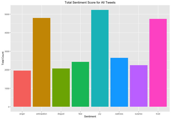
I am a positive person on Twitter, apparently, with joy, anticipation, and trust far outweighing the other emotions. Now let’s see if the sentiment of my tweets has changed over time. We can use dplyr and cut to group the tweets into time intervals for analysis.
tweets$timestamp <- with_tz(ymd_hms(tweets$timestamp), "America/Chicago")
posnegtime <- tweets %>%
        group_by(timestamp = cut(timestamp, breaks="2 months")) %>%
        summarise(negative = mean(negative),
                  positive = mean(positive)) %>% melt
names(posnegtime) <- c("timestamp", "sentiment", "meanvalue")
posnegtime$sentiment = factor(posnegtime$sentiment,levels(posnegtime$sentiment)[c(2,1)])

ggplot(data = posnegtime, aes(x = as.Date(timestamp), y = meanvalue, group = sentiment)) +
        geom_line(size = 2.5, alpha = 0.7, aes(color = sentiment)) +
        geom_point(size = 0.5) +
        ylim(0, NA) +
        scale_colour_manual(values = c("springgreen4", "firebrick3")) +
        theme(legend.title=element_blank(), axis.title.x = element_blank()) +
        scale_x_date(breaks = date_breaks("9 months"),
                     labels = date_format("%Y-%b")) +
        ylab("Average sentiment score") +
        ggtitle("Sentiment Over Time")
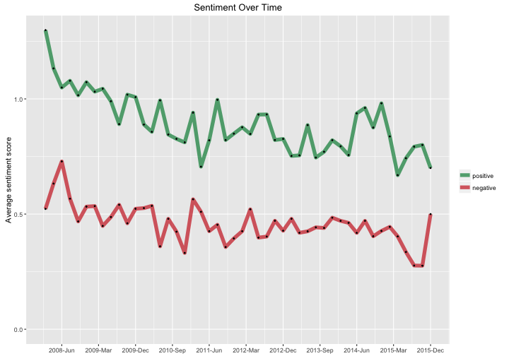
The positive sentiment scores are always much higher than the negative sentiment scores, but both show some decrease over time. The positive sentiment exhibits a stronger downward trend. Apparently, I am gradually becoming less exuberant in my vocabulary on Twitter?
Now let’s see if there are any associations between day of the week and the emotions from the NRC lexicon. Use the wday() function from the lubridate package and dplyr to group the tweets by weekday.
tweets$weekday <- wday(tweets$timestamp, label = TRUE)
weeklysentiment <- tweets %>% group_by(weekday) %>%
        summarise(anger = mean(anger),
                  anticipation = mean(anticipation),
                  disgust = mean(disgust),
                  fear = mean(fear),
                  joy = mean(joy),
                  sadness = mean(sadness),
                  surprise = mean(surprise),
                  trust = mean(trust)) %>% melt
names(weeklysentiment) <- c("weekday", "sentiment", "meanvalue")

ggplot(data = weeklysentiment, aes(x = weekday, y = meanvalue, group = sentiment)) +
        geom_line(size = 2.5, alpha = 0.7, aes(color = sentiment)) +
        geom_point(size = 0.5) +
        ylim(0, 0.6) +
        theme(legend.title=element_blank(), axis.title.x = element_blank()) +
        ylab("Average sentiment score") +
        ggtitle("Sentiment During the Week")
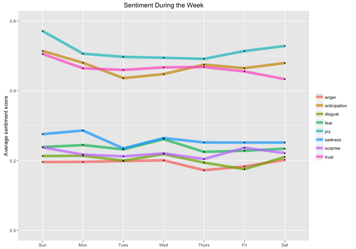
These are mostly consistent with being flat, although it looks like joy and anticipation may be higher on the weekends than on weekdays.
Similarly, let’s see if there are associations between the eight emotions and the months of the year.
tweets$month <- month(tweets$timestamp, label = TRUE)
monthlysentiment <- tweets %>% group_by(month) %>%
        summarise(anger = mean(anger),
                  anticipation = mean(anticipation),
                  disgust = mean(disgust),
                  fear = mean(fear),
                  joy = mean(joy),
                  sadness = mean(sadness),
                  surprise = mean(surprise),
                  trust = mean(trust)) %>% melt
names(monthlysentiment) <- c("month", "sentiment", "meanvalue")

ggplot(data = monthlysentiment, aes(x = month, y = meanvalue, group = sentiment)) +
        geom_line(size = 2.5, alpha = 0.7, aes(color = sentiment)) +
        geom_point(size = 0.5) +
        ylim(0, NA) +
        theme(legend.title=element_blank(), axis.title.x = element_blank()) +
        ylab("Average sentiment score") +
        ggtitle("Sentiment During the Year")
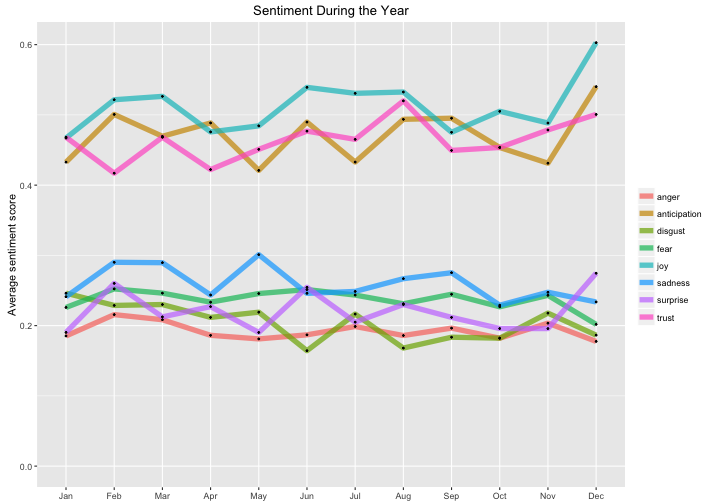
The first thing to notice here is that the variance is much higher for the months of the year than it was for the days of the week. Most (all?) of this must be from our old friend, the Central Limit Theorem. The sample size used to calculate each point is about 12/7 bigger for the plot showing the days of the week compared to the plot showing the months of the year, so we would expect the variance to be 12/7 (or 1.714) times larger in the months-of-the-year plot. Another thing I notice is that joy and anticipation show a distinct increase in December. May your December also be full of joy and anticipation!
The End
The R Markdown file used to make this blog post is available here. I am happy to hear feedback and suggestions; these are some very powerful packages I used in this analysis and I know I only scratched the surface of the kind of work that can be done with them.