Measuring Gobbledygook
By Julia Silge
November 25, 2016
In learning more about text mining over the past several months, one aspect of text that I’ve been interested in is readability. A text’s readability measures how hard or easy it is for a reader to read and understand what a text is saying; it depends on how sentences are written, what words are chosen, and so forth. I first became really aware of readability scores of books through my kids’ reading tracking websites for school, but it turns out there are lots of frameworks for measuring readability.
One of the most commonly used ways to measure readability is a SMOG grade, which stands for “Simple Measure of Gobbledygook”. It may have a silly (SILLY WONDERFUL) name, but it is often considered the gold standard of readability formulas and performs well in many contexts. We calculate a SMOG score using the formula
\[\text{SMOG} = 1.0430\sqrt{\frac{30n_{\text{polysyllables}}}{n_{\text{sentences}}}} + 3.1291\]
where the number in the numerator measures the number of words with 3 or more syllables and the number in the denominator measures the number of sentences. You can see that SMOG is going to be higher for texts with a lot of words with many syllables in each sentence. These ratios are typically normalized to use a sample of 30 sentences, and then the SMOG grade is supposed to estimate the years of education needed to understand a text.
This seems like it is perfectly suited to an analysis using tidy data principles, so let’s use the tidytext package to compare the readability of several texts.
Getting some texts to analyze
Let’s use the gutenbergr package to obtain some book texts to compare. I want to compare:
- Anne of Green Gables by L. M. Montgomery
- Little Women by Louisa May Alcott
- Pride and Prejudice by Jane Austen (I mean, DUH)
- A Portrait of the Artist as a Young Man by James Joyce
- Les Misérables by Victor Hugo
library(gutenbergr)
books <- gutenberg_download(c(45, 514, 42671, 4217, 135),
                            meta_fields = "title")
I really wanted to throw some Ernest Hemingway in there, but none of his works are on Project Gutenberg; I guess they are not public domain.
Tidying the text
Now we have our texts in hand, and we need to do some data wrangling to get it in the form that we need. We are interested in counting two things here:
- the number of sentences
- the number of words with 3 or more syllables
Let’s start by working with the sentences. The unnest_tokens function in tidytext has an option to tokenize by sentences, but it can have trouble with UTF-8 encoded text, lots of dialogue, etc. We need to use iconv first on the UTF-8 text from Project Gutenberg before trying to tokenize by sentences. Also, we have three different books in this dataframe, so we need to nest and map so that we count sentences separately for each book; unnest_tokens will collapse all the text in a dataframe together before tokenizing by something like sentences, n-grams, etc.
library(dplyr)
library(tidytext)
library(tidyr)
library(purrr)

tidybooks <- books %>%
    mutate(text = iconv(text, to = 'latin1')) %>%
    nest(-title) %>%
    mutate(tidied = map(data, unnest_tokens, 'sentence', 'text', token = 'sentences'))
It still takes me a bit of thinking and experimenting every time I need to nest and map, but what a great way to do what I need! How did this work out?
tidybooks## # A tibble: 5 x 3
## title data tidied
## <chr> <list> <list>
## 1 Anne of Green Gables <tibble [10,779 x 2]> <tibble [7,383 x 2]>
## 2 Les Misérables <tibble [67,273 x 2]> <tibble [35,682 x 2]>
## 3 Little Women <tibble [20,627 x 2]> <tibble [10,117 x 2]>
## 4 A Portrait of the Artist as a Young Man <tibble [9,938 x 2]> <tibble [4,583 x 2]>
## 5 Pride and Prejudice <tibble [13,311 x 2]> <tibble [6,951 x 2]>The data column contains the original untidied text and the tidied column contains the tidied text, organized with each sentence on its own row; both are list-columns. Now let’s unnest this so we get rid of the list-columns and have sentences in their own rows.
tidybooks <- tidybooks %>%
    unnest(tidied)

tidybooks
## # A tibble: 64,716 x 3
## title gutenberg_id
## <chr> <int>
## 1 Anne of Green Gables 45
## 2 Anne of Green Gables 45
## 3 Anne of Green Gables 45
## 4 Anne of Green Gables 45
## 5 Anne of Green Gables 45
## 6 Anne of Green Gables 45
## 7 Anne of Green Gables 45
## 8 Anne of Green Gables 45
## 9 Anne of Green Gables 45
## 10 Anne of Green Gables 45
## # ... with 64,706 more rows, and 1 more variables: sentence <chr>How did the sentence tokenizing do?
tidybooks %>%
    sample_n(5) %>%
    select(sentence)
## # A tibble: 5 x 1
## sentence
## <chr>
## 1 "\"i am certainly the most fortunate creature that ever existed!\""
## 2 the assassinated man who flees is more suspicious than the assassin, and it is probable that this personage, who had been so precious a capture for th
## 3 she has more the air of a bat than of a lark.
## 4 all at once he took off his hat and placed it on the edge of the quay.
## 5 it was not a combat, it was the interior of a furnace; there mouths breathed the flame; there countenances were extraordinary.Pretty well! Especially considering the whole thing errors out without iconv.
Now we know how to count the number of sentences in each book.
tidybooks %>%
    group_by(title) %>%
    summarise(n_sentences = n_distinct(sentence))
## # A tibble: 5 x 2
## title n_sentences
## <chr> <int>
## 1 A Portrait of the Artist as a Young Man 4480
## 2 Anne of Green Gables 7176
## 3 Les Misérables 34229
## 4 Little Women 9888
## 5 Pride and Prejudice 6524There we go! An estimate of the number of sentences in each book.
Counting syllables
The next thing we need to do here is count the syllables in each word so that we can find how many words in each book have more than 3 syllables. I did a bit of background checking on how this is done, and found this implementation of syllable counting by Tyler Kendall at the University of Oregon. It is actually an implementation in R of an algorithm originally written in PHP by Greg Fast, and it seems like a standard way people do this. It is estimated to have an error rate of ~15%, and is usually off by only one syllable when it is wrong.
I’m including this function in a code chunk with echo = FALSE because it is really long and I didn’t write it, but you can check out the R Markdown file that made this blog post to see the details.
Let’s check out how it works!
count_syllables("dog")## [1] 1count_syllables("science")## [1] 2count_syllables("couldn't")## [1] 2count_syllables("My name is Julia Silge.")## [1] 7Well, my last name is actually two syllables, but most human beings get that wrong too, so there we go.
Now let’s start counting the syllables in all the words in our books. Let’s use unnest_tokens again to extract all the single words from the sentences; this time we will set drop = FALSE so we keep the sentences for counting purposes. Let’s add a new column that will count the syllables for each word. (This takes a bit to run on my fairly speedy/new desktop; that function for counting syllables is not built for speed.)
tidybooks <- tidybooks %>%
    unnest_tokens(word, sentence, drop = FALSE) %>%
    rowwise() %>%
    mutate(n_syllables = count_syllables(word)) %>%
    ungroup()

tidybooks %>%
    select(word, n_syllables)
## # A tibble: 1,070,066 x 2
## word n_syllables
## <chr> <dbl>
## 1 anne 1
## 2 of 1
## 3 green 1
## 4 gables 2
## 5 by 1
## 6 lucy 2
## 7 maud 1
## 8 montgomery 4
## 9 table 2
## 10 of 1
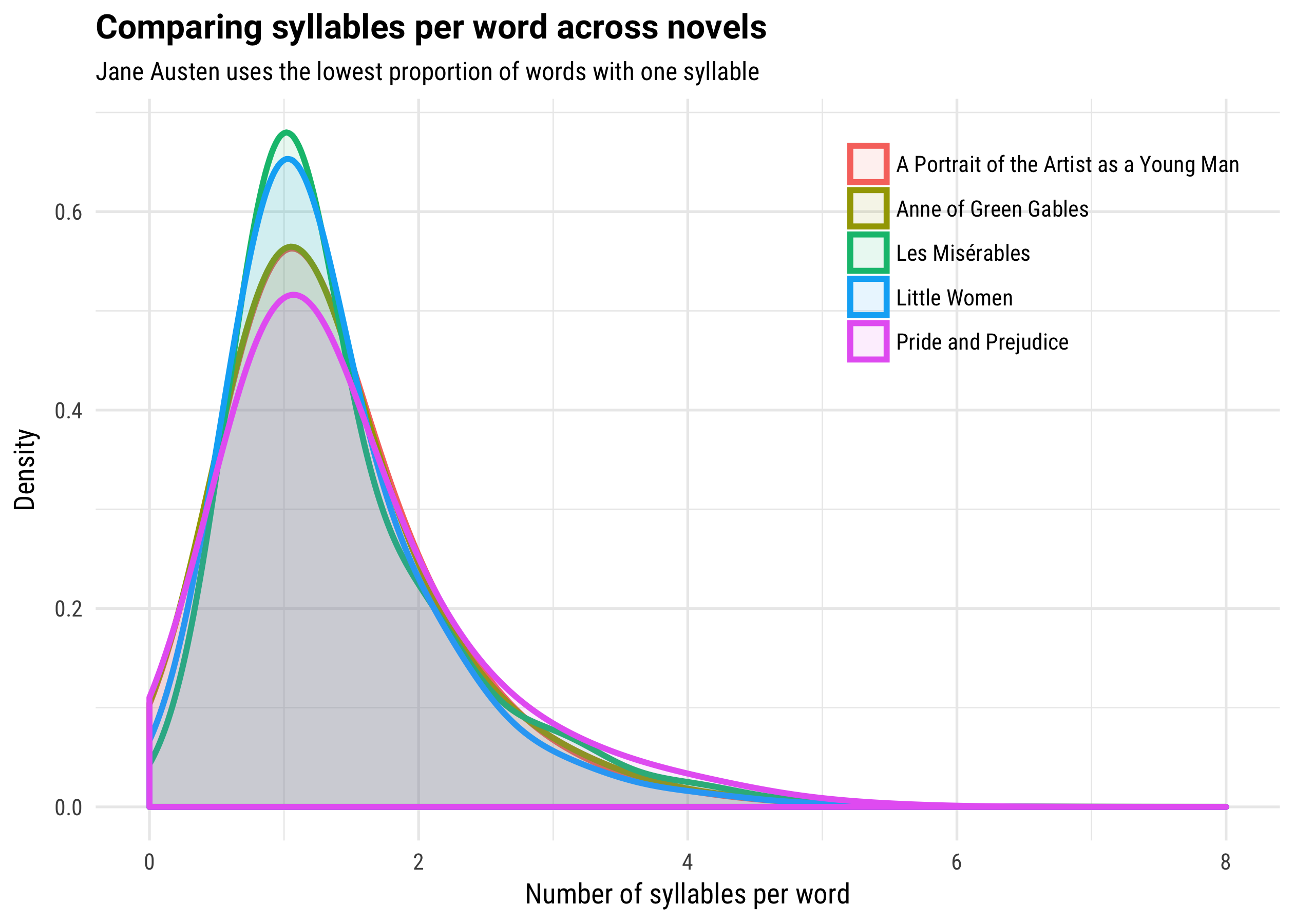
## # ... with 1,070,056 more rowsLet’s check out the distributions of syllables for the three titles.
library(ggplot2)
ggplot(tidybooks, aes(n_syllables, fill = title, color = title)) +
    geom_density(alpha = 0.1, size = 1.1, adjust = 9) +
    theme_minimal(base_family = "RobotoCondensed-Regular") +
    theme(plot.title=element_text(family="Roboto-Bold")) +
    theme(legend.title=element_blank()) +
    theme(legend.position = c(0.8, 0.8)) +
    labs(x = "Number of syllables per word",
         y = "Density",
         title = "Comparing syllables per word across novels",
         subtitle = "Jane Austen uses the lowest proportion of words with one syllable")
These distributions are pretty similar, but there are some moderate differences. Little Women and Les Misérables have the highest proportion of words with only one syllable, while Pride and Prejudice has the lowest proportion. This makes some sense, since Louisa May Alcott was writing for young readers while Jane Austen was not. Les Misérables was originally written in French and we are analyzing a translation here, so that is a complicating factor. James Joyce, with his moocows or whatever, is in the middle here.
Calculating SMOG
Now we know both the number of sentences and the number of syllables in these books, so we can calculate… the gobbledygook! This will just end up being a bunch of dplyr operations.
results <- left_join(tidybooks %>%
                         group_by(title) %>%
                         summarise(n_sentences = n_distinct(sentence)),
                     tidybooks %>%
                         group_by(title) %>%
                         filter(n_syllables >= 3) %>%
                         summarise(n_polysyllables = n())) %>%
    mutate(SMOG = 1.0430 * sqrt(30 * n_polysyllables/n_sentences) + 3.1291)

results
## # A tibble: 5 x 4
## title n_sentences n_polysyllables SMOG
## <chr> <int> <int> <dbl>
## 1 A Portrait of the Artist as a Young Man 4480 5648 9.543459
## 2 Anne of Green Gables 7176 7664 9.032898
## 3 Les Misérables 34228 55114 10.378218
## 4 Little Women 9888 11590 9.313996
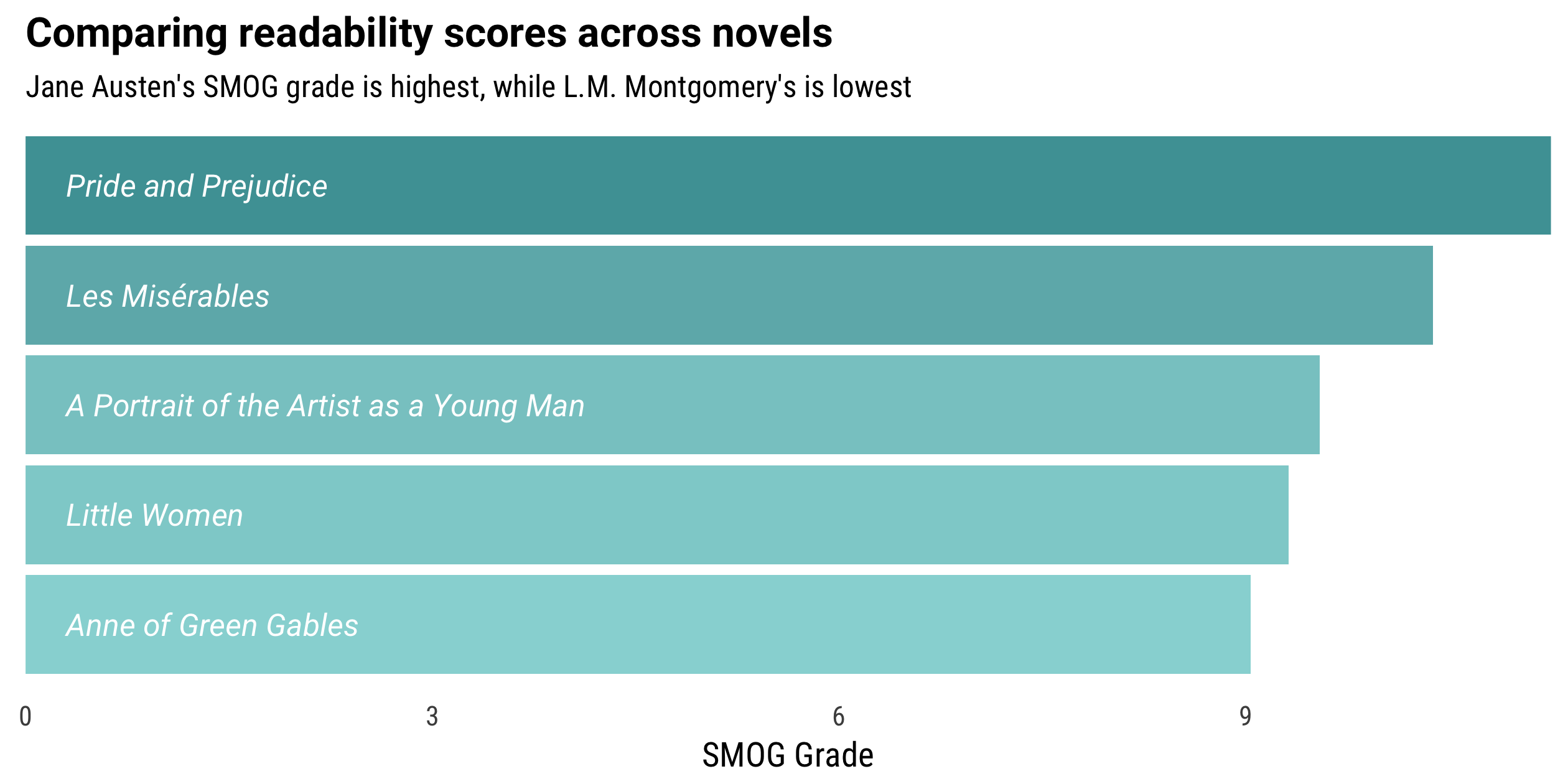
## 5 Pride and Prejudice 6524 13180 11.248906L.M. Montgomery, writing here for an audience of young girls, has the lowest SMOG grade at around 9 (i.e., approximately beginning 9th grade level). Pride and Prejudice has the highest SMOG grade at 11.2, more than two years of education higher. I will say that throwing A Portrait of the Artist as a Young Man in here turned out to be an interesting choice; in reality, I find it to be practically unreadable but it has a readability score close to the same as Little Women. This measure of prose readability based only on number of sentences and number of words with lots of syllables doesn’t measure what we might expect when applied to extremely stylized text.
Let’s visualize the readability scores for these five novels.
library(ggstance)
library(ggthemes)
library(forcats)
ggplot(results, aes(SMOG, fct_reorder(title, SMOG), fill = SMOG)) +
    geom_barh(stat = "identity", alpha = 0.8) +
    theme_tufte(base_family = "RobotoCondensed-Regular") +
    geom_text(aes(x = 0.3, y = title, label = title), color="white",
                  family="Roboto-Italic", size=3.5, hjust = 0) +
    theme(plot.title=element_text(family="Roboto-Bold")) +
    scale_fill_gradient(low = "darkslategray3", high = "turquoise4") +
    theme(legend.position="none") +
    theme(axis.ticks=element_blank()) +
    scale_x_continuous(expand=c(0,0)) +
    theme(axis.text.y=element_blank()) +
    labs(y = NULL, x = "SMOG Grade",
         title = "Comparing readability scores across novels",
         subtitle = "Jane Austen's SMOG grade is highest, while L.M. Montgomery's is lowest")
The End
I would like to thank Ben Heubl, a data journalist at The Economist, for interesting discussions that motivated this blog post. The R Markdown file used to make this blog post is available here. I am very happy to hear feedback or questions!