Use racing methods to tune xgboost models and predict home runs

This is the latest in my series of screencasts demonstrating how to use the tidymodels packages, from just getting started to tuning more complex models. This week’s episode of SLICED, a competitive data science streaming show, had contestants compete to predict home runs in recent baseball games. Honestly I don’t know much about baseball ⚾ but the finetune package had a recent release and this challenge offers a good opportunity to show how to use racing methods for tuning.

Here is the code I used in the video, for those who prefer reading instead of or in addition to video.

Explore data

Our modeling goal is to predict whether a batter’s hit results in a home run given features about the hit. The main data set provided is in a CSV file called training.csv.

library(tidyverse)
train_raw <- read_csv("train.csv")

You can watch this week’s full episode of SLICED to see lots of exploratory data analysis and visualization of this dataset, but let’s just make a few plots to understand it better.

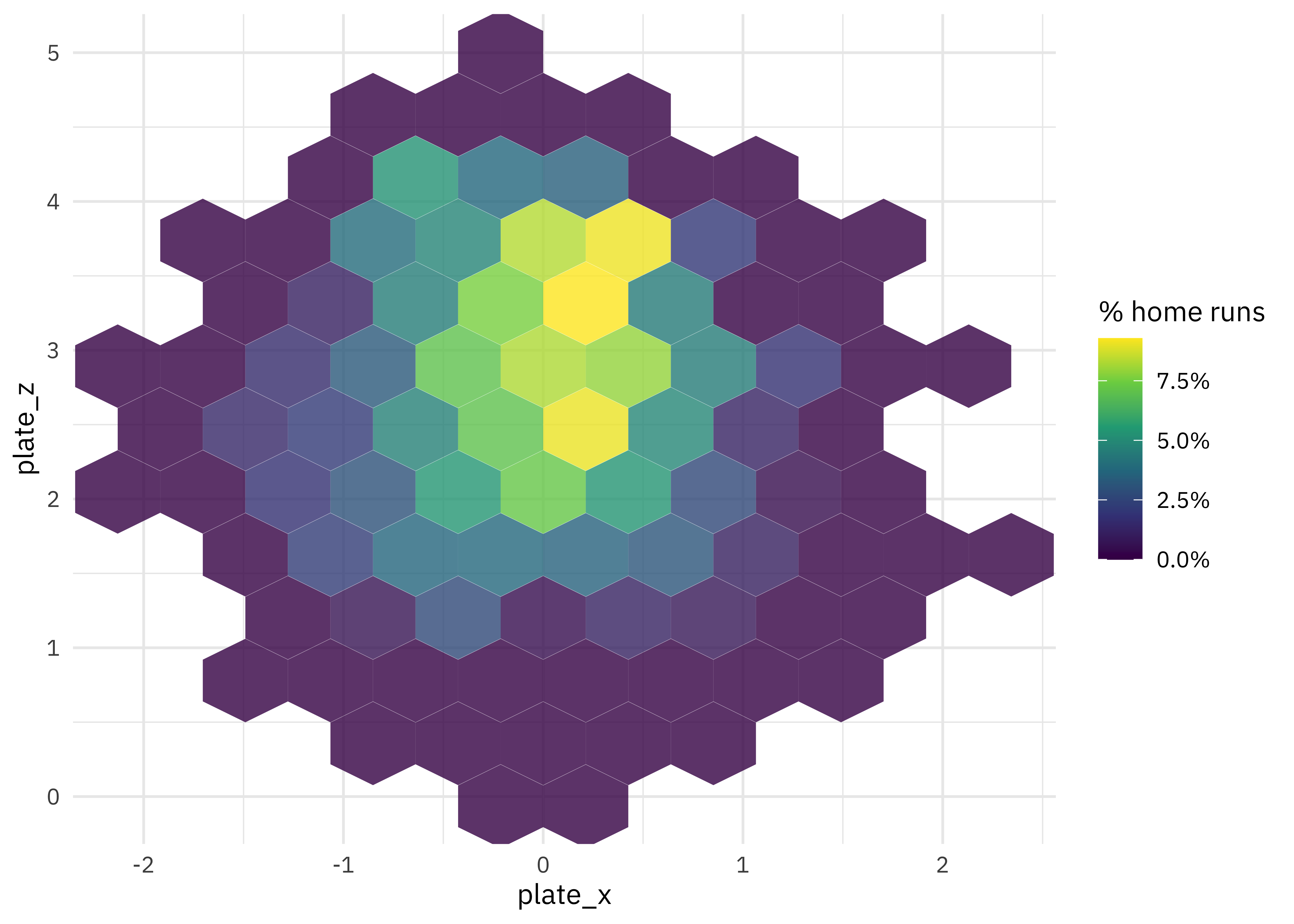
How are home runs distributed in the physical space around home plate?

train_raw %>%
  ggplot(aes(plate_x, plate_z, z = is_home_run)) +
  stat_summary_hex(alpha = 0.8, bins = 10) +
  scale_fill_viridis_c(labels = percent) +
  labs(fill = "% home runs")

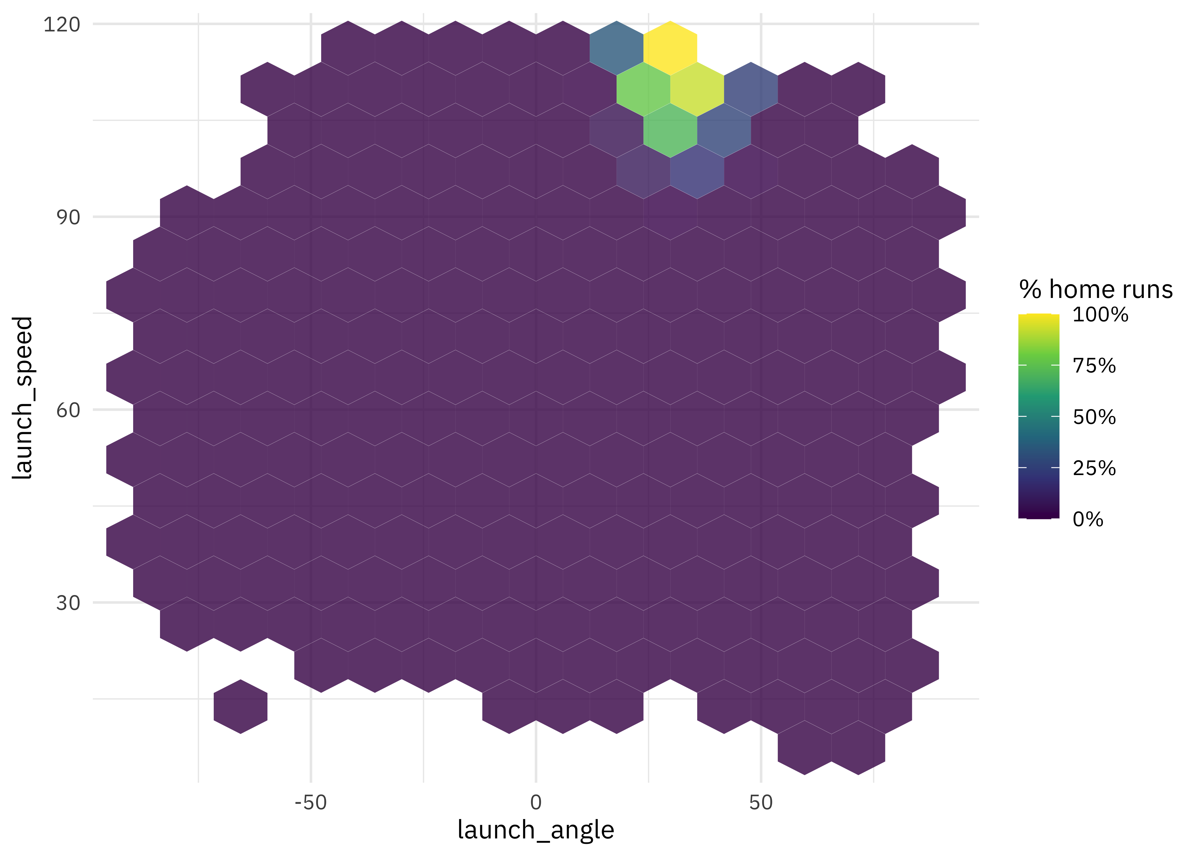
How do launch speed and angle of the ball leaving the bat affect home run percentage?

train_raw %>%
  ggplot(aes(launch_angle, launch_speed, z = is_home_run)) +
  stat_summary_hex(alpha = 0.8, bins = 15) +
  scale_fill_viridis_c(labels = percent) +
  labs(fill = "% home runs")

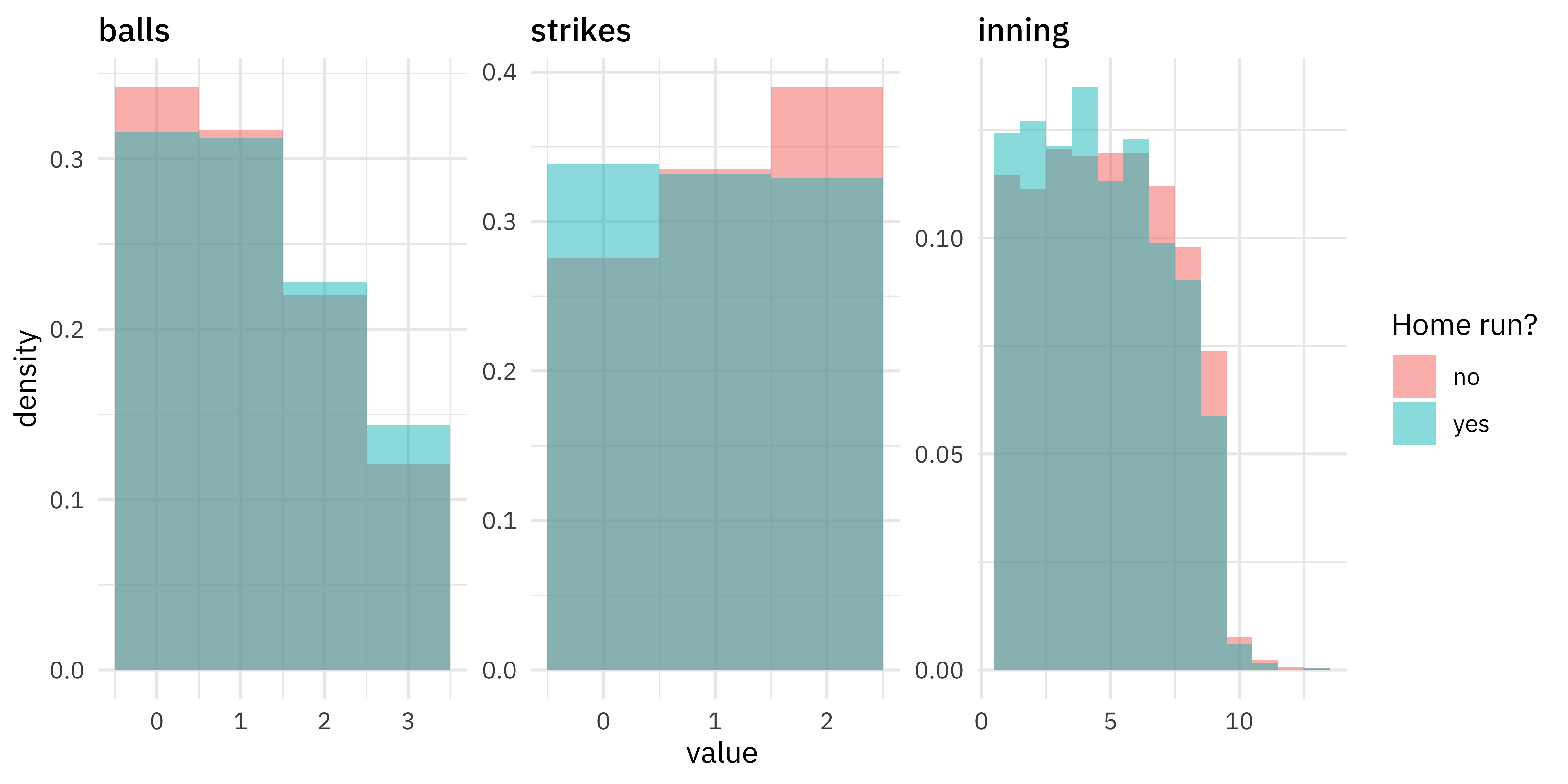
How does pacing, like the number of balls, strikes, or the inning, affect home runs?

train_raw %>%
  mutate(is_home_run = if_else(as.logical(is_home_run), "yes", "no")) %>%
  select(is_home_run, balls, strikes, inning) %>%
  pivot_longer(balls:inning) %>%
  mutate(name = fct_inorder(name)) %>%
  ggplot(aes(value, after_stat(density), fill = is_home_run)) +
  geom_histogram(alpha = 0.5, binwidth = 1, position = "identity") +
  facet_wrap(~name, scales = "free") +
  labs(fill = "Home run?")

There is certainly lots more to discover, but let’s move on to modeling.

Build a model

Let’s start our modeling by setting up our “data budget.” I’m going to convert the 0s and 1s from the original dataset into a factor for classification modeling.

library(tidymodels)

set.seed(123)
bb_split <- train_raw %>%
  mutate(
    is_home_run = if_else(as.logical(is_home_run), "HR", "no"),
    is_home_run = factor(is_home_run)
  ) %>%
  initial_split(strata = is_home_run)
bb_train <- training(bb_split)
bb_test <- testing(bb_split)

set.seed(234)
bb_folds <- vfold_cv(bb_train, strata = is_home_run)
bb_folds

## #  10-fold cross-validation using stratification 
## # A tibble: 10 × 2
##    splits               id    
##    <list>               <chr> 
##  1 <split [31214/3469]> Fold01
##  2 <split [31214/3469]> Fold02
##  3 <split [31214/3469]> Fold03
##  4 <split [31215/3468]> Fold04
##  5 <split [31215/3468]> Fold05
##  6 <split [31215/3468]> Fold06
##  7 <split [31215/3468]> Fold07
##  8 <split [31215/3468]> Fold08
##  9 <split [31215/3468]> Fold09
## 10 <split [31215/3468]> Fold10

For feature engineering, let’s concentrate on the variables we already explored during EDA along with info about the pitch and handedness of players. There is some missing data, especially in the launch_angle and launch_speed, so let’s impute those values.

bb_rec <-
  recipe(is_home_run ~ launch_angle + launch_speed + plate_x + plate_z +
    bb_type + bearing + pitch_mph +
    is_pitcher_lefty + is_batter_lefty +
    inning + balls + strikes + game_date,
  data = bb_train
  ) %>%
  step_date(game_date, features = c("week"), keep_original_cols = FALSE) %>%
  step_unknown(all_nominal_predictors()) %>%
  step_dummy(all_nominal_predictors(), one_hot = TRUE) %>%
  step_impute_median(all_numeric_predictors(), -launch_angle, -launch_speed) %>%
  step_impute_linear(launch_angle, launch_speed,
    impute_with = imp_vars(plate_x, plate_z, pitch_mph)
  ) %>%
  step_nzv(all_predictors())

## we can `prep()` just to check that it works
prep(bb_rec)

## Data Recipe
## 
## Inputs:
## 
##       role #variables
##    outcome          1
##  predictor         13
## 
## Training data contained 34683 data points and 15255 incomplete rows. 
## 
## Operations:
## 
## Date features from game_date [trained]
## Unknown factor level assignment for bb_type, bearing [trained]
## Dummy variables from bb_type, bearing [trained]
## Median Imputation for plate_x, plate_z, pitch_mph, ... [trained]
## Linear regression imputation for launch_angle, launch_speed [trained]
## Sparse, unbalanced variable filter removed bb_type_unknown, bearing_unknown [trained]

Now let’s create a tunable xgboost model specification. In a competition like SLICED, we likely wouldn’t want to tune all these parameters because of time constraints, but instead only some of the most important.

xgb_spec <-
  boost_tree(
    trees = tune(),
    min_n = tune(),
    mtry = tune(),
    learn_rate = 0.01
  ) %>%
  set_engine("xgboost") %>%
  set_mode("classification")

xgb_wf <- workflow(bb_rec, xgb_spec)

Use racing to tune xgboost

Now we can use tune_race_anova() to eliminate parameter combinations that are not doing well. This particular SLICED episode was being evaluted on log loss.

library(finetune)
doParallel::registerDoParallel()

set.seed(345)
xgb_rs <- tune_race_anova(
  xgb_wf,
  resamples = bb_folds,
  grid = 15,
  metrics = metric_set(mn_log_loss),
  control = control_race(verbose_elim = TRUE)
)

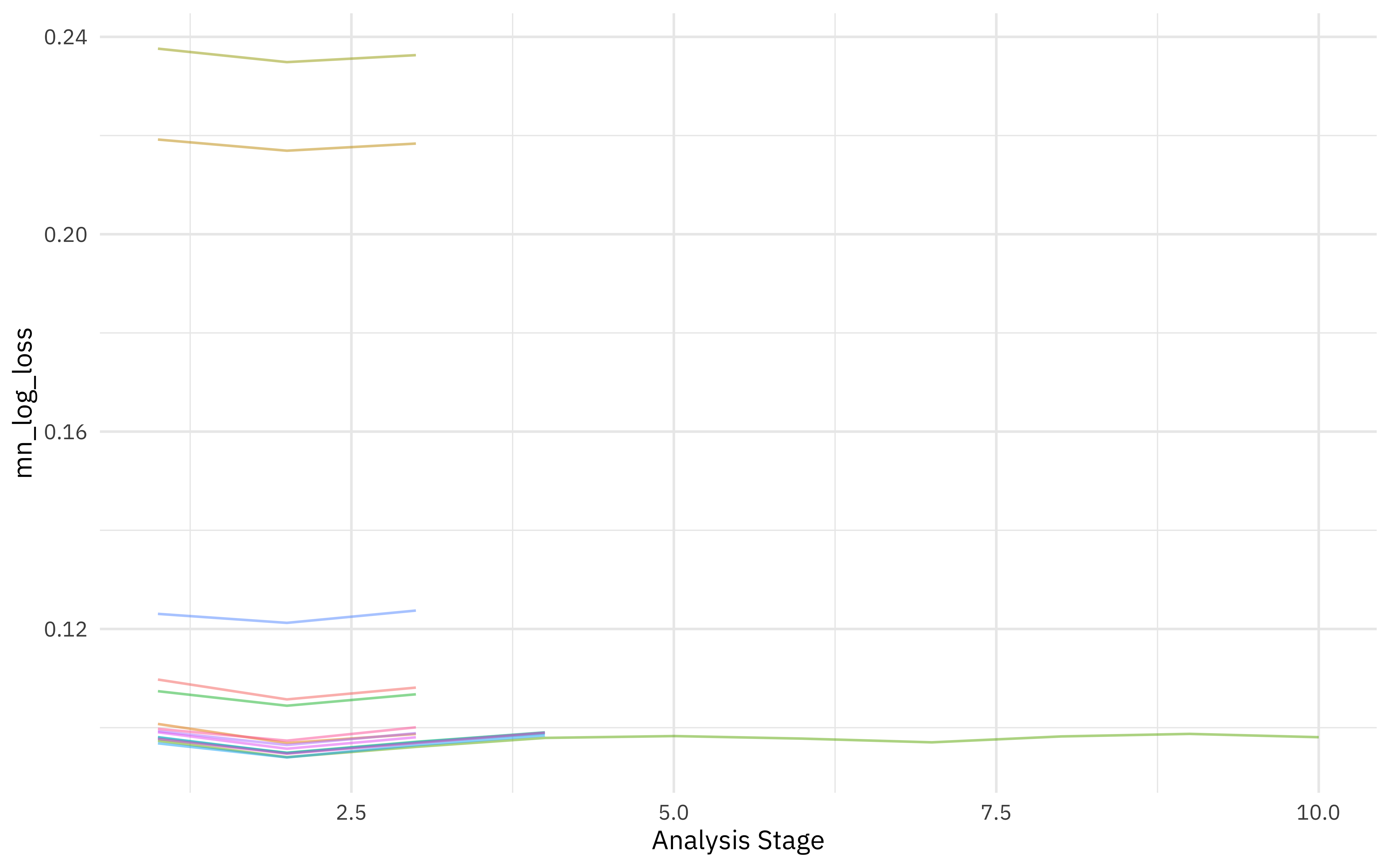
We can visualize how the possible parameter combinations we tried did during the “race.” Notice how we saved a TON of time by not evaluating the parameter combinations that were clearly doing poorly on all the resamples; we only kept going with the good parameter combinations.

plot_race(xgb_rs)

And we can look at the top results.

show_best(xgb_rs)

## # A tibble: 1 × 9
##    mtry trees min_n .metric    .estimator   mean     n std_err .config          
##   <int> <int> <int> <chr>      <chr>       <dbl> <int>   <dbl> <chr>            
## 1     6  1536    11 mn_log_lo… binary     0.0981    10 0.00171 Preprocessor1_Mo…

Let’s use last_fit() to fit one final time to the training data and evaluate one final time on the testing data.

xgb_last <- xgb_wf %>%
  finalize_workflow(select_best(xgb_rs, "mn_log_loss")) %>%
  last_fit(bb_split)

xgb_last

## # Resampling results
## # Manual resampling 
## # A tibble: 1 × 6
##   splits         id          .metrics     .notes      .predictions     .workflow
##   <list>         <chr>       <list>       <list>      <list>           <list>   
## 1 <split [34683… train/test… <tibble [2 … <tibble [0… <tibble [11,561… <workflo…

We can collect the predictions on the testing set and do whatever we want, like create an ROC curve, or in this case compute log loss.

collect_predictions(xgb_last) %>%
  mn_log_loss(is_home_run, .pred_HR)

## # A tibble: 1 × 3
##   .metric     .estimator .estimate
##   <chr>       <chr>          <dbl>
## 1 mn_log_loss binary        0.0975

This is pretty good for a single model; the competitors on SLICED who achieved better scores than this using this dataset all used ensemble models, I believe.

We can also compute variable importance scores using the vip package.

library(vip)
extract_workflow(xgb_last) %>%
  extract_fit_parsnip() %>%
  vip(geom = "point", num_features = 15)

Using racing methods is a great way to tune through lots of possible parameter options more quickly. Perhaps I’ll put it to the test next Tuesday, when I participate in the second and final episode of the SLICED playoffs!